How to Avoid Software Cost and Schedule Overruns

How successful are software projects today? To find out, you may want to ask your favorite AI agent. I asked Copilot to provide statistics on software project schedule, effort, and cost outcomes compared to plans.

 

 

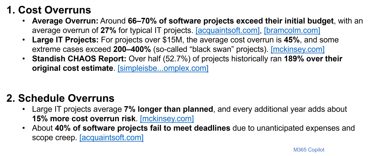
The accuracy of these numbers may be questionable, but the overall message is not. Software project cost and schedule overruns abound! Measuring software size throughout the software project lifecycle provides the insights you need to reduce risk and improve software project success.

Up to this point in our Software Size Matters video series, we have covered the benefits of quantifying software size and presented sizing metrics and methods that fit the type of software development work you do. In this episode, we present examples of how to apply these concepts throughout the project lifecycle.

 

 

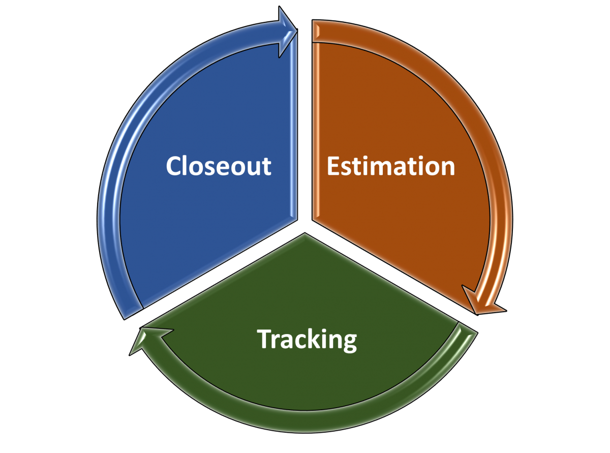
Quantifying software size is an important best practice for each of the three major project stages:

• Estimation: producing scope-based Rough Order of Magnitude (ROM) estimates to support feasibility assessments at the initiation and planning stages, and detailed estimates to support project commitments.
• Tracking: as the scope is better understood and features are completed, comparing planned versus actual software size completed to get a true picture of in-process project status and forecasting estimates to complete.
• Closeout: capturing completed project data to expand and refine data analytics, provide a basis of estimation of future projects, and conduct performance benchmarking to support process improvement initiatives and establish competitive positions.

 

 

 

Estimation Stage

Much of the material covered in previous Software Size Matters videos emphasized the importance of using software size metrics to estimate software project scope, because cost, effort, team size, quality, and productivity all increase nonlinearly with software size. In Episode 4, Choosing a Sizing Method, we discussed the benefits of estimating software project scope using T-shirt sizing early in the lifecycle when the scope is not well defined. More accurate estimates are generated from scope-based T-shirt sizes than from effort or cost-based T-shirt sizes.
 

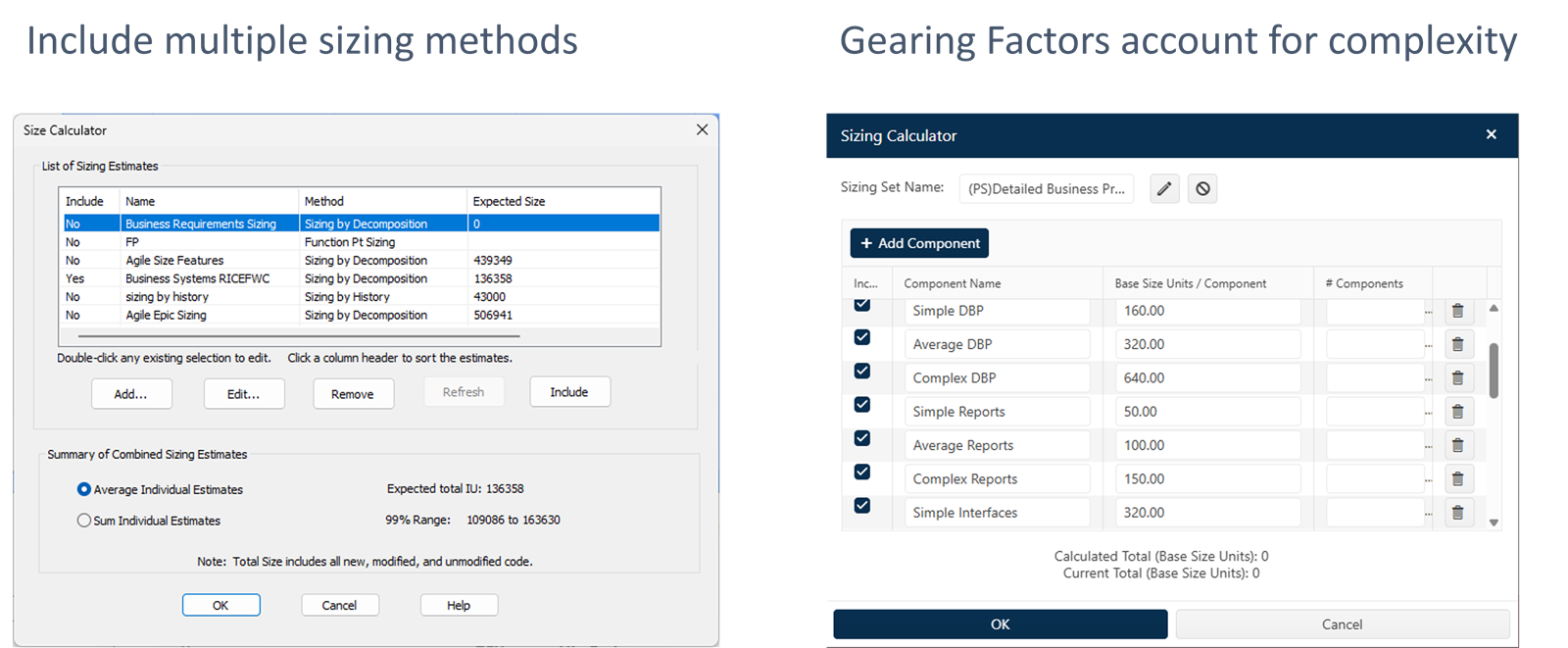
Once the software requirements are understood, detailed size estimates can be calculated using one or more methods. In Episodes 4 and 5, we discussed the variety of software sizing methods and the associated function units you can use that fit the data you have available and the type of work you do. We suggest using multiple sizing methods to reduce uncertainty. You can compare the results from each method, select one, or average them. Using different gearing factors for small, average, and complex function units, like Reports and Interfaces in this example, not only increases the accuracy of software size estimates, but also promotes stakeholder participation in the process. Subject matter experts can help select the best size bin for each component.

 

Tracking Stage

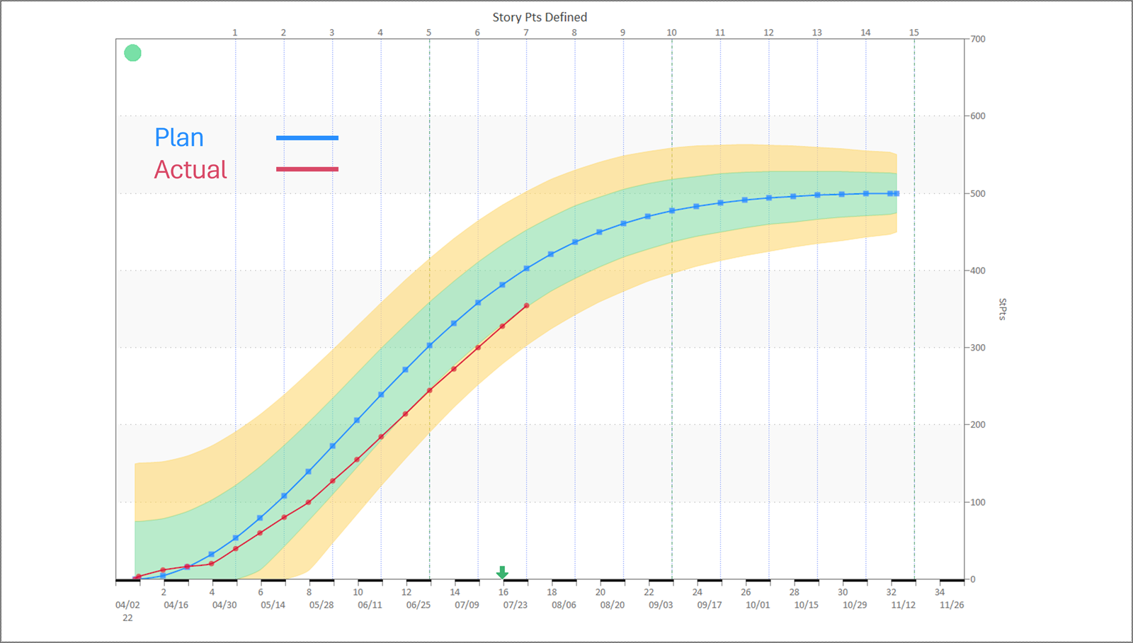
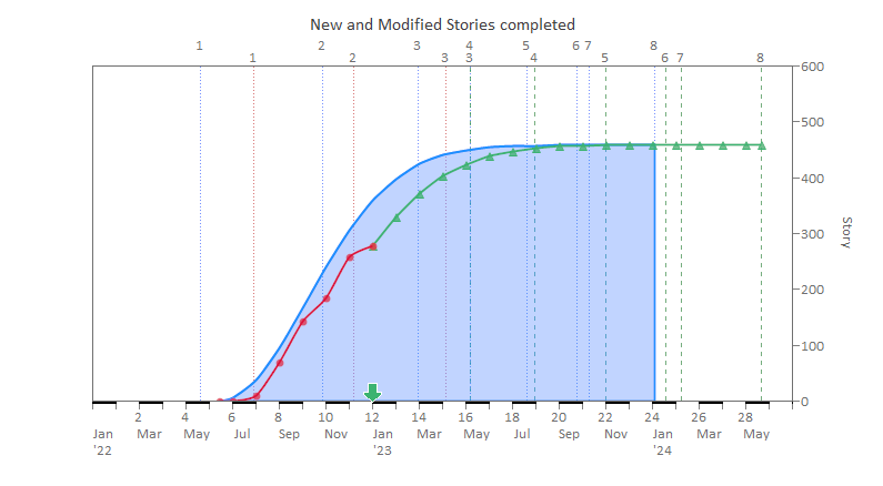
It is essential to continue to use software size metrics to track the progress of ongoing software projects. Actual software size metrics are the best indicator of project status. You can see the rate at which work is being done and the cumulative to date compared to your plan. Schedule, effort, and staffing metrics are helpful, but they only tell you what resources have been expended, not what work has been completed. Many organizations employing Agile methods use product backlog buildup or drawdown charts. The chart below shows that the cumulative number of Story Points Defined has been under plan for several sprints (indicated by the vertical dotted lines). This type of insight provides early warnings so corrective action and replanning can be done to either meet schedule and cost targets or renegotiate commitments.

 

 

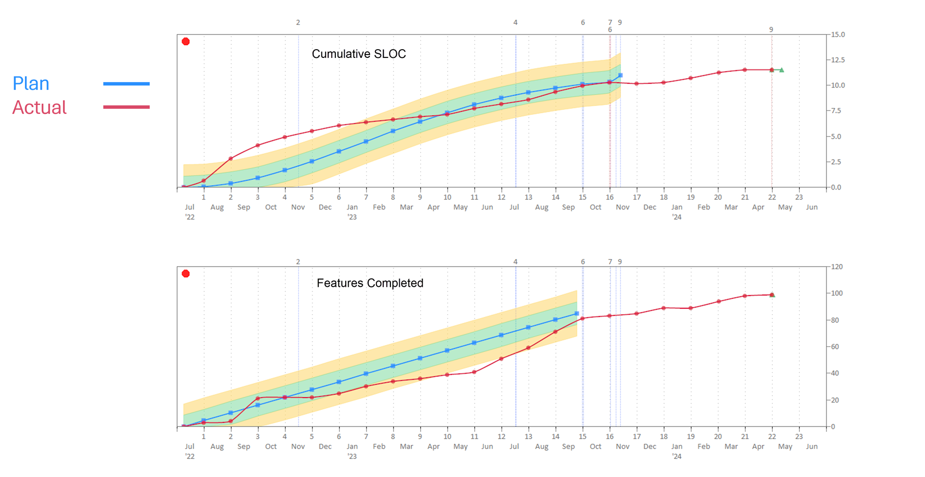
Tracking plan versus actual data for multiple size metrics will provide interesting and valuable insights. We estimated the planned number of Source Lines of Code (SLOC) and Features to be delivered for one of our projects. Some things we observed are:

• The SLOC count was much higher than planned in the beginning months, while the Features were slightly under. This was because some architectural framework development needed to be done before Features could be completed.
• Actual SLOC counts showed steady progress consistent with the plan in the latter half of the project.
• All Features were assumed to be of average size and able to be completed at regular intervals. Notice the straight line buildup of the blue plan line. We didn't have information to assign Features to size bins. The relative size and dependency among different Features can mean you don't get to take credit for completing them at regular intervals.
• The SLOC count proved to be a more accurate predictor of project status for this project.
• The Feature counts helped us improve our size estimates for the next release.

 

 

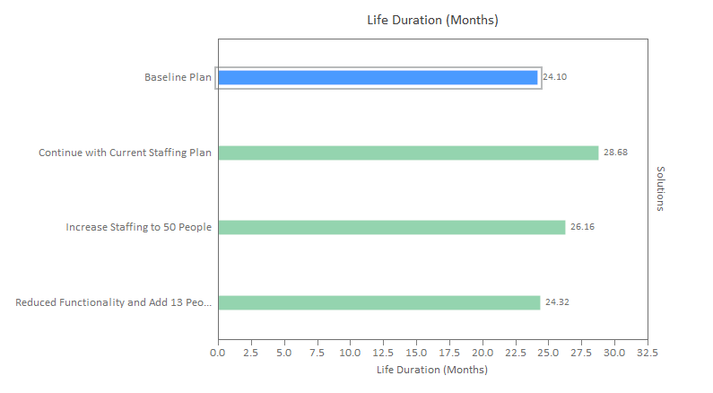
The really great thing about tracking actual software size is that you can run curve fit forecasts for size metrics to calculate the expected completion date. If you are also tracking plan versus actual effort, which most organizations do, you can compute your actual productivity. QSM's process productivity measure (Productivity Index) captures the overall project environment efficiency, not just development teams, making it a reliable basis for forecasting to completion.

 

 

A good practice is to run “What-if?” forecasts to account for scope creep or potential changes in other key indicators, like increasing staff or having to mitigate product quality issues. That way, you can see the impact and risks of alternative scenarios and update plans accordingly.

 

 

Closeout Stage

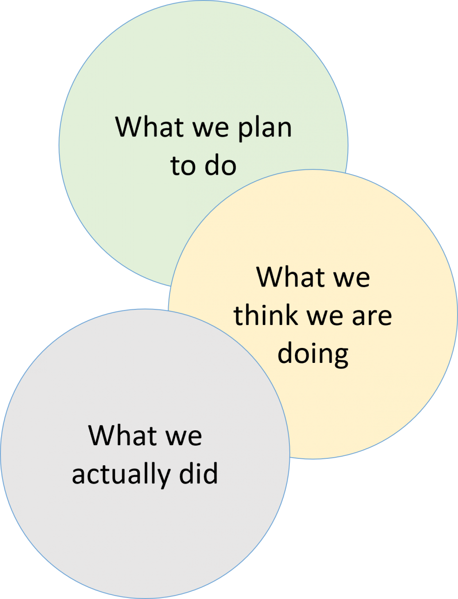
Software projects don't always turn out exactly how we planned! Ideally, what we plan to do, what we think we are doing, and what we actually did would show a high degree of overlap. Most organizations want historical performance data but haven't dedicated time or resources to this discipline.

Here are a few reasons for collecting historical data:

• It promotes good record-keeping and supports the use of AI tools. Not only do we have bad memories, but we also have selective memory. We need reliable data about software project outcomes to train and use artificial intelligence and promote data-driven decision-making.
• It's used to develop software development performance benchmarks. Some of our customers are software vendors who bid on proposals and need to show that they are the best in the software industry. Others are organizations evaluating vendor bids using performance benchmarks to identify risky offers.
• It accounts for variations in cost and schedule performance. Analyzing your historical data enables you to answer questions like “Was productivity down because of staffing issues?” for example.
• It supports statistically validated trends and analysis. QSM software project history trends are valuable, but the best practice is to produce custom trends from your data.
• It makes software estimates defensible. Software estimates based on historical data reduce the impact of personal emotions and business politics by letting the data speak.
• It is used to bound productivity assumptions. Productivity is slow to change. Productivities you measure for certain project types today will be relevant for some time. There are no silver bullets.

 

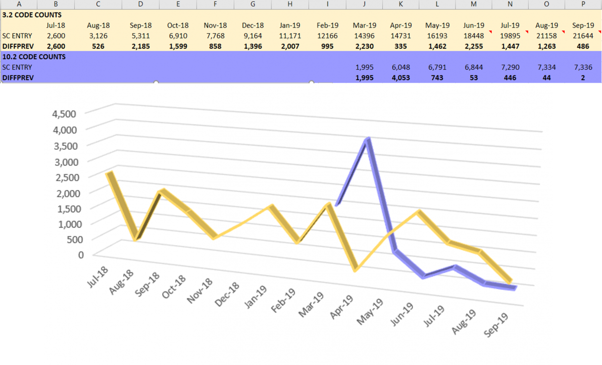
Historical data helps you recognize patterns. The slide below shows the monthly actual Source Lines of Code (SLOC) counts for two different QSM projects. The code count we measure is cumulative because that is the easiest to extract from our software configuration management application. You can use any size unit if you can't get code counts. We started computing the monthly production rate by calculating the difference in cumulative values as shown in the chart below. We can identify values that seem out of whack with the normal production rate of each project. That's a signal to investigate and find out if we made a data manipulation error, the code counting script includes something new, or what the cause may be. Data validation checks are necessary! Note the wide variation in monthly coding rates. Context about the project is important. Variation may reflect any of the following:

• Staffing changes.
• Multitasking or time-slicing between projects, as shown by the April numbers.
• Feature complexity.
• Partially finished work, meaning you may not be able to check in software code until it's done-done.
• Where you are in the project lifecycle, for example, tailing off at the end of the project, beginning in June.
• Or scope creep − last-minute additions.

 

 

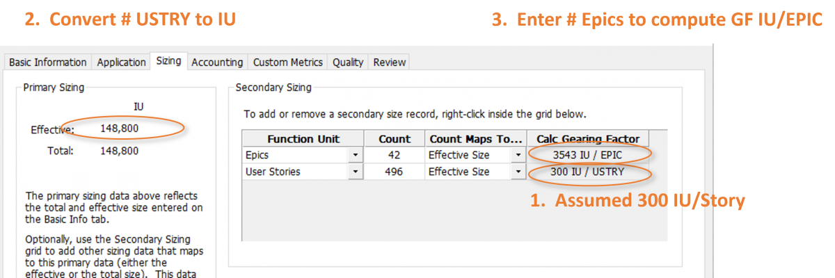
In Episode 5 of this video series, we presented the concept of using Gearing Factors to convert Function Units to a common Base Size Unit for project comparisons and capturing feature complexity in size estimates. You can compute Gearing Factors for the function units you use when you have SLOC counts. You say, “Laura, that's really awesome, but there's no way I can get a code count.” OK, here's another approach that works:

• First, select a similar function unit for which you have data. In this case, we assumed a Gearing Factor of 300 Implementation Units (IU) per User Story based on work that we did for several clients.
• Next, we multiplied the Gearing Factor times the number of User Stories completed, in this case 496, to calculate the Base Size Unit in IUs.
• Then we were able to use that number to compute an average Gearing Factor for EPICs: 3543 IU per EPIC. Now the EPIC and User Story data can be used to define the T-shirt sizes for ROM estimates of future software projects.

 

 

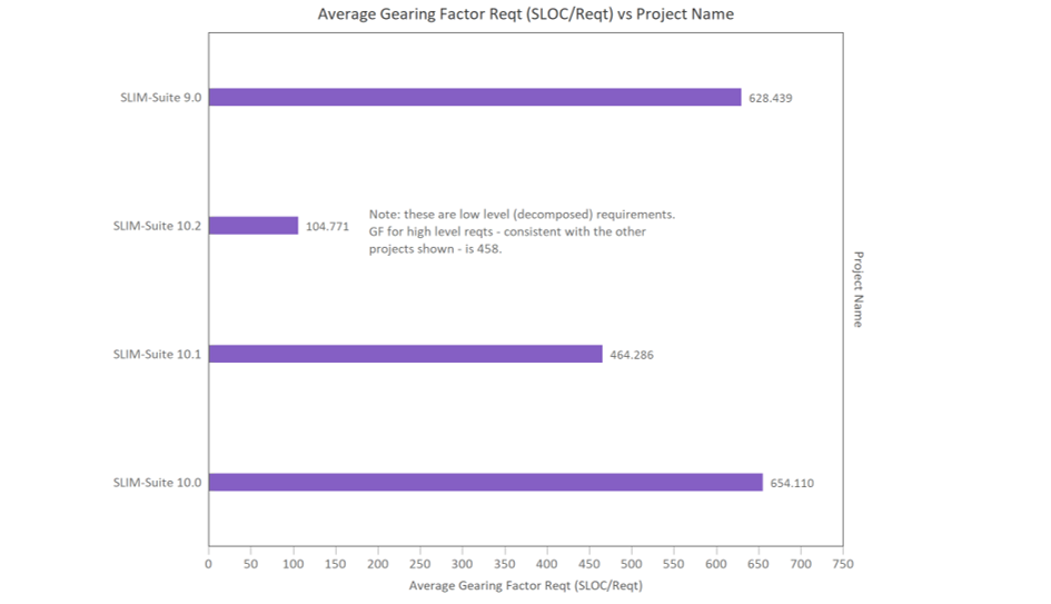
Different projects may have different Gearing Factors for the same software unit, depending upon the rigor, formality, and consistency of your software metrics process. The chart below shows software Requirement Gearing Factors (SLOC/Requirement) for different releases of the same application. Versions 9.0 and 10.0 were very consistent. On average, each requirement resulted in a big change, indicated by the high Gearing Factor, and thus, required more work. It won’t take long for you to recognize patterns in your work.

 

 

To summarize, quantifying software size is key to successfully navigating every stage of the software project lifecycle.

• During Estimation, software size is the best predictor of software project schedule, effort, staffing, cost, and quality outcomes.
• During Tracking, software size measures provide a true picture of project status and a realistic basis for forecasts.
• During Closeout, software size measures calibrate predictive models and provide insights for understanding project dynamics, and it also guides process improvement initiatives.

In this video, we looked at the benefits of quantifying software size throughout the project lifecycle. I hope you'll join me for our final video, Benchmarking and Estimation Validation.