Frequently Asked Questions

I set a Schedule Constraint of 24 months. Why does the Solution Panel show a 22-month schedule for the life cycle?

There are several reasons this could be happening, but the most likely cause is that you entered a target probability of more than 50% for the Schedule constraint. For example, if you enter a time constraint of 24 months at a target probability of 90%, you are asking SLIM-Estimate to calculate a risk-buffered solution that provides a 90% probability that the project will not exceed 24 months: in effect, a risk-buffered solution.

The difference between the expected solution of 22 months (50%) and your constraint of 24 months (90%) represents the built-in risk buffer that protects you against possible size growth, lower than estimated productivity, staff availability issues, or other facts that may affect the delivery date. The size of this risk buffer is determined by the uncertainty range around the estimated size, PI, and manpower buildup.  The Solution Panel always displays the 50% solution because it is the work plan.

If you want your solution to correspond exactly to your input constraint values, use desired probabilities of 50% for those constraints.

What is the difference between the Base Size Unit and the Function Unit?

The Function Unit is a measure of software size, which represents the project scope or the amount of work to be done.  It makes sense to dscribe a book as a collection of chapters, or a building by the number of floors or rooms it contains.  The Function Unit allows us to describe a system as a group of functional or logical components, e.g., Function Points, features, reports, or interfaces.

The QSM database contains thousands of projects sized in different Function Units.  Without a common reference point it would be impossible to make meaningful size comparisons between a project sized in Function Point to one sized in User Stories.  The Base Size Unit represents the most common, elementary programming steps being  performed.  Historically, that was writing lines of code and labeled Source Lines of Code (SLOC).  With the introduction of modern development tools, a more generic term, Implementation Unit (IU) was added to account for tasks such as configuring packages or using a GUI interface to build a cloud infrastructure.  To normalize the Function Units to the Base Size Unit so project data can be used in scatter plots for comparison and to create statistical trend lines, we need a conversion, or Gearing Factor that tells us how big components are relative to each other.  For example, a common Gearing Factor for Functions Points is 50 IU/FP - on average it takes 50 programming steps to implement 1 Function Point.

The Base Size Unit is set by going to Tools | Customize Global Options.  Choose the acronym that reflects the work being performed - typically IU or SLOC.  The Gearing Factor of the Base Size Unit is always 1 - it cannot be set the the user.

The Function Unit is set by going to Tools | Customize Project Environment, Project Environment tab.  In the Product Construction area, select the Function Unit that matches the data available or the development method.  In the Agile-Story-Pnt Estimation template installed with SLIM-Estimate, the Function Unit has been set to Story Points with a Gearing Factor of 85 (IU/Story Pnt).  This allows all charts and reports to display the Effective and Total Size in Story Points, which is great for communicating with the Agile community.

Setting the Function Unit to the Base Unit makes it possible to use any number of component types or size units to measure all or parts of the system.  For example, QSM's Package Implementation template contains a Sizing by Decomposition method based on RICEF objects, using different gearing factors for each object type.  This method captures component complexity by supply appropriate gearing factors for simple, average, and complex components like reports and conversions.

If you need help determining an appropriate gearing factor, visit the Function Point Gearing Factors page on the QSM web site, download our Gearing Factors whitepaper, or contact QSM for assistance.

How do I set Phase Start dates?

Phase start dates, duration, and effort settings are used to configure the lifecycle model to your development methods and practices.  Select Estimate | Solution Assumptions from the main menu, then select the Phase Tuning tab.  The start date for the first phase included in the project is the project start date specified on the Solution Assumptions Basic Info tab or via Solution Wizards.

Subsequent phases can be set to begin at:

• Ratio - a specific percentage of the prior phase’s duration (most common)
• Fixed Overlap - a specified number of months into the prior phase
• Specific Date - a specific date.

Select Tuning Factor History... to use phase tuning data from select completed projects loaded in your SLIM-Estimate workbook.

What options are available for sizing projects in SLIM-Estimate?

The Size Calculator offers a variety of sizing techniques that may be used individually or in combination. A common and flexible technique is Sizing by Decomposition, which allows you to break the system down into individual components such as epics, stories, features, RICEF objects, or your custom components, each of which can have its own gearing factor (IU/component). The individual component estimates are rolled up into a total size estimate, which will be posted back to the Solution Assumptions screen.

Instructions for using the Sizing Calculator and descriptions of each sizing method are available in SLIM-Estimate NetHelp.

QSM's Software Size Matters Infographic also provides a great general resource for which sizing unit to use at each point in the software lifecycle.

Please contact QSM Support for help creating your size estimates.

How can I change the unit for Total system size in the Balanced Risk and other solution wizards? Currently it is set to IU, but we use Function Points.

Solution wizards that require a size estimate assumption use the Sizing By History technique to obtain an initial "ballpark" estimate based on the statistical size ranges, or t-shirt sizes, in your project's associated trend group(s).  This technique uses the Function Unit and Gearing Factor in the Project Environment settings.  Most of the templates installed with SLIM-Suite have the Function Unit set to the Base Size Unit, either IU or SLOC.  

To change the Function Unit to Stories, Features, Function Points, or other size unit, select Tools | Customize Project Environment from the menu. On the Project Description Tab, there is a Function Unit list box.  Select Function Points or other unit, then enter an appropriate Gearing Factor to represent the average number of Base Size Units (elementary programming steps) contained in your selected  Function Unit (ex.: a gearing factor of 50 represents 50 Base Size Units per Function Point).  

If you need help determining an appropriate gearing factor, visit the Function Point Gearing Factors page on the QSM web site, download our Gearing Factors whitepaper, or contact QSM for assistance.

Though we provide "starter" skills allocation for both new workbooks and QSM templates, the skills breakout is turned off by default because the skill categories, labor rates, and skills allocation data are most meaningful when they are configured to match the roles and practices actually in use on your projects. We recommend you create a template or two that represents a typical project resource requirement schema for your organization, then tailor it for individual projects as necessary.  

The Configuration Options tab of the Refine Resources/Costs/Skills dialog contains a field where you can specify a maximum percentage of fixed personnel for each time period.  If you enter a “50”, SLIM-Estimate automatically scales back the fixed resources to comply with specified percentage.  In this case, the total number of fixed personnel in a given month will never exceed 50%.  For each time period, the max resource effort hours are subtracted from the total effort for that time period, then percentage-based skills allocation settings are applied to the remaining monthly effort.

The planned MTTD value shown on my graph for the final month of phase 3 is not the same as the value reported in the Project Profile report and the consistency report for my Phase 3 MTTD. It appears to be slightly higher in the reports.  Why?

The value displayed on graphs is the average MTTD rate for the final month of phase 3, but the MTTD value reported in the reports represents the planned MTTD at the end of phase 3. You should expect this value to be somewhat higher than the average value for the entire month, because the theoretical MTTD is always improving (getting larger) as time progresses.

I changed my runtime environment from 5 days to 7 days. I would have expected my MTTD value to get smaller because I am running the system longer. Why did my MTTD value get larger?

The MTTD value is simply the reciprocal of the monthly defect rate. Suppose the expected defect rate is 100 defects found during the last month of phase 3. This is a theoretical monthly rate number based on an average runtime environment. The MTTD for this month is therefore 1 month/100 errors or .01 months between defects. 

Because it is difficult to think in terms of .01 months, you can specify a more intuitive MTTD time unit.  If you select days, then .01 months is the same as .01 * 30 (roughly) or .3 days between defects (assuming you are running 7 days a week). However, if you are running only 5 days a week, then .01 months converts to (.01 * 20) or .2 days.

The Solution Panel says my peak staff value is 10.3, but the Average Staffing Rate charts and reports show a peak staff of 10.1. What is causing this inconsistency?

The theoretical Rayleigh curve used to derive the values on the Solution Panel is a smooth curve resulting in different staffing numbers at each point along the x-axis. In drawing the Average Staffing chart, this smooth theoretical curve is approximated by a series of discrete staffing rates (with one bar, or average staffing rate value, per month).

The graph and solution panel values won't always match exactly because the graphical peak staff is always taken mid-month for any internal month while the solution panel always shows the highest peak staff point on the staffing curve (regardless of when it occurs). Usually the theoretical curve does not peak exactly at mid-month, so the true peak shown on the solution panel will not match the one on the average staffing charts unless the theoretical peak happens to fall at mid-month.

On large projects where a longer schedule allows a natural smoothing of the staffing curve, the theoretical peak staff will usually be close to the average staff rate value. On shorter projects, you can expect to see larger discrepancies.

Sometimes the effort data points on my Life Cycle Sensitivity to PI graph have values that do not always increase (or decrease); e.g., there are small dips in the data.

Remember that the time and effort shown on these graphs are life cycle values. The most likely cause of slight variations in the expected behavior of the data is caused by variation in the effort for phase 4. Staffing projections for phase 4 are dependent on the staffing rate at the end of phase 3. Therefore, differences in the final phase 3 staffing rate can result in variations in the total effort for phase 4. You can check to see if this is the case by making the solutions in question the current solution, then comparing the phase 4 effort in the solution panel of the staffing view.

The 50% solution is based on the expected value (the solution with a 50% probability of achieving the same or better values for schedule, effort, cost, and reliability). Each of the inputs to an estimate - size, application complexity, and productivity - has some uncertainty associated with it. If any one of your input parameters (size, for instance) increases significantly from the original estimate, it makes sense that the actual outcome will vary from the estimated outcome.

To manage this uncertainty, SLIM-Estimate employs the concept of a risk-buffered solution. The estimate or “work plan” is a 50% probability solution. If the project is managed to this 50% solution, the risk charts should reflect alternative delivery dates at various levels of assurance. You can decide which date to promise to the customer based on your risk tolerance and your assessment of the amount of uncertainty in your inputs.

Essentially, the time difference between the 50% delivery date and the 90% (or whatever assurance level you choose) delivery date represents the amount of schedule buffer needed to account for the possibility that one or more of your input parameters will vary significantly from the estimate.

The alternate outcomes on each risk chart are based on the assumption that the 50% solution represents the work plan for the project. If the project is worked to another plan (the 70% assurance solution, for instance), the values on the risk charts will change.

When I change the Person Hours per Person Month field on the Accounting tab of the Solution Assumptions dialog, there is no change to the total schedule and effort for the project. Why is this?

Many SLIM-Estimate and SLIM-Control users have asked why their overall schedule does not change when they change the value of the "Person Hours per Person Month" field,  Solution Assumptions screen, Accounting Tab.

The number of Person Hours comprising a particular organization's Person Month is not used to calculate total effort.  If your chosen effort unit is Person Months, the hours per month setting is not used at all. If, on the other hand, your effort unit is weeks, days, or hours, your hours per month will be used to convert the estimated total effort (in Person Months) into your chosen effort unit.

At first, this may seem counter-intuitive. Shouldn't an increase or decrease in the number of Person Hours in a Person Month be reflected in the final estimate?

The number of staff hours in an organization's staffing month is more relevant in the accounting world than it is in software estimation. It attempts to account for items such as vacations, meetings, and administrative activities but in most cases, it is merely an estimate or average.  It may tell how many hours will be charged to a particular project, but has nothing to say about how much is actually accomplished during those hours (or even how many actual hours were worked). The productivity index, or PI, is where actual work produced is measured.

The Productivity Index, or PI, reflects a number of environmental factors such as:

If you are using a PI calculated from your past projects, your user-specified PI already reflects the conditions in your working environment. Holding other factors constant, organizations which have high "administrative overhead" will tend to have a lower calculated productivity index than organizations which maximize time spent working on the most productive project tasks.

SLIM-Estimate® is a macro model based on the software equation described in Measures for Excellence. The SLIM software equation is designed to estimate consistently across a broad spectrum of working environments and accounting standards. For this reason, the effort parameter was originally calculated in Person Years, which are converted to Person Months in SLIM-Estimate. Once the total effort in PM has been determined, it can be converted into your chosen effort unit for display on charts and reports.  But what if you have no historical data and are using the PI suggested by the QSM database? SLIM estimating and project control tools will still give you a good first estimate that you can continue to refine as more project data becomes available. As projects are completed, SLIM tools will calculate the project PI's from your historical data. These PI's can be used to calibrate new estimates to the unique conditions in your development environment.

As you begin to compare and analyze PI's from completed projects, you can spot and eliminate bottlenecks as well as identify successful strategies that you can repeat to improve productivity. Storing project metrics in a useful and accessible form and analyzing them to identify trends is the key to process and productivity improvement. Consistent use of SLIM tools results in increasingly accurate estimates and will help you build a repository of historical data for future analysis and benchmarking.

What is the purpose of the gearing factor?

Gearing factors are used to convert projects with many different sizing units (objects, modules, or use cases for example) back to a common sizing unit: the Basic Work Unit. The Basic Work Unit represents the smallest sizing unit that is common to all projects.

This conversion is important for two reasons. First, it allows us to apply the same family of PIs (or Productivity Indices) to all projects. Second, it allows you to compare your project, whether it is sized in tables, screens, or any other sizing unit, to QSM’s industry – or your own custom - trend lines, which can be sized in a variety of size units.

In our research, we have found a strong correlation between system size and important metrics like PI, schedule, effort, and defects. For more information on gearing factors, download our free whitepaper.

The Installation and Deployment section of the QSM Resource Library web page provides System Requirements, step by step installation instructions, and other useful information about SLIM-Suite.

Information on the latest version of SLIM-Suite (along with download links, release notes, and installation instructions) can be found on the Installation and Upgrades page of the QSM website.  To see whether you're running the latest version, select Help | Check for updates from the menu of any SLIM-Suite application.

Often SLIM-Suite license renewals do not correspond with new product releases.  To update the license information for your current SLIM-Suite installation, use Windows Control Panel | Programs and Features application utililty.  Select the appropriate QsmTools installation (e.g. QsmTools 10.3) and right-click and choose Change.  Select Modify on the Install Shield screen and follow the prompts to enter your new Registration Code and Activation Code(s).  Review the list of products to be installed to ensure they match your license agreement.

No.  When the server copy of SLIM-Suite is updated, all users are automatically upgraded to the same version of SLIM-Suite.  No further action is needed on your part.

We update our function point gearing factors table every few years. Formal releases of our database and over 600 industry trend lines are followed by updates to resources like the gearing factors table. For a variety of reasons, it’s not practical to update continually.

Typically, new projects are submitted in small batches. Out of any given group of projects, only a very small subset are suitable for use in the table (recent, medium or high confidence, single language FP projects). Updating too frequently would result in only trivial changes to the table, but would make the job of checking a variety of previous tables with continually changing values quite a bit harder.

Finally, it makes sense to work with largest possible data set when updating our published values. This is only possible given sufficient time for large data samples to be collected and validated and for the data to be carefully analyzed and reviewed. In the mean time, if you have a question or don't see a language you're interested in, don't hesitate to contact QSM support.  

Access to our industry database of over 13,000 completed software projects is included in your license!

Here's how to locate your SLIM license information:

• If the applications are already installed:
  • Simply launch any SLIM application and look at the right side of the splash screen, or
  • With the application open, select Help | About SLIM... from the menu to access the splash screen.

• If your license has expired or the application has not been installed yet, try the following:
  •  If the application is installed on your computer, simply browse to the directory where it is installed (Usually C:\Program Files\QSM\Toolsnn, where “nn” is the current version of SLIM-Suite). To determine the path to the application directory, right-click on the application shortcut and select the "properties" tab. Locate the readme.txt file located in your Toolsnn folder. Open this file in Notepad or any other text editor - it contains your license information.
  • If the applications have not yet been installed, contact the software administrator for your company and ask for a copy of your license email.
  • If you need help locating your software administrator or license email (or if you have questions) call QSM at 800 424-6755 for assistance.

What are the latest versions of the SLIM Tool Suite?

Information on the latest version of SLIM-Suite (along with download links, release notes, and installation FAQs) can be found on the Downloads page of the QSM website. To see whether you're running the latest version, select Help | Check for updates from the menu of any SLIM-Suite application.

In SLIM-Suite, some dialog boxes are too large for my screen.  What is the recommended screen resolution?

If you are running at a low screen resolution, certain dialog boxes may not fit within the screen display. 

The recommended screen resolution is 1024 x 768 with 256 colors and 96 dpi (default small fonts). For optimal graphics display when running SLIM tools, the screen resolution should be set to at least 800 by 600 for small fonts (or at a higher resolution if you are using large fonts). 

There's a good fit between my total defect data and the plan but in the defects by category charts, the defect actuals for each category aren't tracking the plan very well. How can I fix this?

Chances are your defect category percentages need to be adjusted. To tune these percentages using your actual data, create a Multi-Metric Time Series Chart and insert a QSM Tracked Defects Category Total (Actual) metric for each defect category you're tracking:

Next, right click on your chart to access the chart property tabs. On the Data tab, select "Percent of first metric's data points" and click OK to exit the dialog.

Next, toggle your Multi-Metric chart into report form:

If the weekly or monthly values seem fairly consistent, you can simply use the latest % of total for each category. If you see a lot of variation, you may want to average the values - don't be afraid to experiment until you get the best visual fit! Enter the % for each category on the Reliability tab of the Project Environment dialog:

Once you return to the defects by category views, you should see a better fit between the plan and actuals.

Can I use the forecast function to explore various staffing options?

When you run a forecast, SLIM-Control bases the future staffing profile on the peak staff and staffing shape defined in the current plan.

While Phase 3 is ongoing, run a tradeoff forecast to see the impact of increasing or decreasing staff and apply any resulting schedule tradeoff to your existing forecast.  To run a tradeoff forecast, select Control | Tradeoff Forecast… from the menu.

Once Phase 3 has completed, use the maintenance forecast to evaluate staff tradeoffs.  The maintenance forecast can only be performed during Phase 4.  To run a maintenance forecast, select Control | Run Forecast… from the menu.

My current plan is extremely inconsistent with my actual data. For instance, the project started a year late and has already slipped by almost 15 months.  Using my original plan, the actual defect data yields a defect tuning factor of 2000% when I run the Defect Tuning Calculator function. 

Is the plan being factored into the defect tuning calculations? If so, can significant variation between the plan and the actuals result in an incorrect tuning factor?

When looking for the best tuning factor, SLIM-Control must make some assumptions in order to generate a set of theoretical defect curves and find the one that best fits your actual data. If these assumptions are incorrect (for example, if either the expected phase 3 duration or expected effort are wrong) then any calculations based on these assumptions will be affected. 

Before running the Defect Tuning Calculator, it’s a good idea to review the current plan to ensure reasonable consistency with your actual data. If your actuals have diverged significantly from the current plan, it should be updated before defect tuning is performed. To update the current plan, run a forecast, make the forecast the current plan, then re-run the Defect Tuning Calculator. 

Sometimes, one or more of the menu items in SLIM-Control are grayed out and I'm not sure why.

Grayed out menu options generally denote features that will not become available until some condition has been satisfied. Here are some of the most common reasons a menu option may be unavailable:

1.     You're trying to edit a QSM Default custom metric or control bound. Since QSM default custom metrics and control bound definitions cannot be edited, the options for these metrics are grayed out. You can, however,  copy a QSM default metric or control bound definition and edit the copy.

2.     You're trying to enter actual data for a metric that has not started yet or is complete. Before you can enter actual data for a metric, you must first enter an actual start date for that metric. Likewise, once you've entered an actual end date for a metric, you will no longer be able to enter actual data for that metric. 

3.     You're trying to set a start or end date for a metric that is tied to a phase:  Start and end date fields for planned staffing/effort are disabled because staffing and effort data is always tied to a specific phase. For example, phase 2 effort begins on the first day of phase 2 and ends on the last day of phase 2. Start/end dates for each phase are defined on the Phases tab of the Plan property sheet (Control | Plan Data). 

Start dates for Defect metrics are customizable, but defect end dates are disabled because they coincide with the end of the life cycle.

4.     You're trying to enter a start or end date for an inactive phase. On the Plan | Phases tab, planned start or end dates can only be entered for active phases. To view/edit the active phases for the project, select Tools | Customize Project Environment and select the Phases tab.

My actual defect data points don't show up on the defect remaining and defect remaining/sloc reports and graphs.   Why not?

Before we can calculate and display the number of errors remaining, we must know the forecasted number of errors in the system.  Planned defects remaining is the difference between planned total defects and planned defects found at various points in time. Actual defects remaining are calculated by subtracting actual defects found from the forecasted total defects.

Therefore, the actual number of defects remaining will be shown only when a forecast exists.

I changed my runtime environment from 5 days to 7 days. I would have expected my MTTD value to get smaller because I am running the system longer. Why did my MTTD value get larger?

The MTTD value is simply the reciprocal of the monthly defect rate. Suppose the expected defect rate is 100 defects found during the last month of phase 3. This is a theoretical monthly rate number based on an average runtime environment. The MTTD for this month is therefore 1 month/100 errors or .01 months between defects. 

Because it is difficult to think in terms of .01 months, you can specify a more intuitive MTTD time unit.  If you select days, then .01 months is the same as .01 * 30 (roughly) or .3 days between defects (assuming you are running 7 days a week). However, if you are running only 5 days a week, then .01 months converts to (.01 * 20) or .2 days.

I sometimes get poor defect curve fits when running a forecast.  What can I do to improve this?

Getting a good curve fit is important - the poorer the fit, the less confidence you will have in the projected new time for that set of data. The goodness of fit is particularly important during the latter stages of Phase 3 because defect data is weighted more heavily at that time. There are two things you can do to improve your defect curve fits:

1.  Assess the reliability of early data points carefully. If you have little confidence in the earliest defect data, you should throw it out. Our theoretical defect data curve algorithm assumes defects are being captured from the start of Phase 3 in a consistent and systematic manner. In practice, however, systematic logging of defects is often not performed until around Systems Integration Test (71% of phase 3 duration). If your early defect data is very erratic, chances are those data points are unreliable. If you know (or suspect) this to be the case, exclude the unreliable data points from curve fitting and forecasting. Unreliable data introduces random noise into SLIM-Control's calculations and creates unreliable forecasts.

2.  Try to determine the best tuning factor for your defect data. This is fairly easy to do once any early noisy data points have been discarded. There are two ways to get a handle on the defect tuning factor.  You can use either one, or combine the two methods:

• The first method uses past projects to generate a historic defect tuning factor. You can use any similar projects captured in SLIM-DataManager. Individual defect tuning factors for each project can be displayed on DataManager’s Project List View by selecting Tools | Customize View Layout from the menu. To get the average Defect Tuning Factor for one or more completed projects, import them into SLIM-Control using the History | Load Projects menu item and then run the Defect Tuning Calculator.  If you plan on using an average DTF from your history, you may wish to inspect the data and eliminate outliers to prevent distortion of the average.
• Once you have entered at least three actual total defect data points into SLIM-Control the Defect Tuning Calculator can also calculate a defect tuning factor from your actual defect data.

Once the expected defect total has been tuned to your history or actual data, you should see an improvement in your defect curve fits. If you’re tracking Defects Found by Category, here's one final step that will help ensure optimal curve fits:

• Tune the % of total defects for each category using your actual data. For more information on how to do this, see the FAQ entitled, "How Do I Tune My Defect Category Percentages?".

If you are still getting poor data fits after performing the steps outlined above, either try to determine the reasons or simply exclude defect data from the forecast curve fit.

The Solution Panel says my peak staff value is 10.3, but the Average Staffing Rate charts and reports show a peak staff of 10.1. What is causing this inconsistency?

The theoretical Rayleigh curve used to derive the values on the Solution Panel is a smooth curve resulting in different staffing numbers at each point along the x-axis. In drawing the Average Staffing chart, this smooth theoretical curve is approximated by a series of discrete staffing rates (with one bar, or average staffing rate value, per month).

The graph and solution panel values won't always match exactly because the graphical peak staff is always taken mid-month for any internal month while the solution panel always shows the highest peak staff point on the staffing curve (regardless of when it occurs). Usually the theoretical curve does not peak exactly at mid-month, so the true peak shown on the solution panel will not match the one on the average staffing charts unless the theoretical peak happens to fall at mid-month.

On large projects where a longer schedule allows a natural smoothing of the staffing curve, the theoretical peak staff will usually be close to the average staff rate value. On shorter projects, you can expect to see larger discrepancies.

How does SLIM-Control handle missing actual data points?

The answer to this question depends on the context. You can display interpolated or missing data points on charts via the "display interpolated data" option in the chart properties. If possible, SLIM-Control will interpolate missing data points using the expected shape of the associated metric curve. Note that only interior data points can be interpolated - SLIM-Control needs a start and end point for interpolation.

It's important to realize that interpolated data points have no bearing on the analysis of actual data in SLIM-Control. When you run a forecast, missing data points are not used during curve fit analysis. The only time missing data is not completely ignored is in the case of milestones. If a milestone should have occurred prior to the projection date (and no actual milestone date has been entered), SLIM-Control assumes the milestone has been missed and the earliest it can occur is immediately after the date of projection. If more than one milestone is "missing", it is assumed that they have all been missed, and that the earliest missed milestone cannot occur before the date of projection.

When I change the Person Hours per Person Month field on the Accounting tab of the Solution Assumptions dialog, there is no change to the total schedule and effort for the project. Why is this?

Many SLIM-Estimate and SLIM-Control users have asked why their overall schedule does not change when they change the value of the "Person Hours per Person Month" field,  Solution Assumptions screen, Accounting Tab.

The number of Person Hours comprising a particular organization's Person Month is not used to calculate total effort.  If your chosen effort unit is Person Months, the hours per month setting is not used at all. If, on the other hand, your effort unit is weeks, days, or hours, your hours per month will be used to convert the estimated total effort (in Person Months) into your chosen effort unit.

At first, this may seem counter-intuitive. Shouldn't an increase or decrease in the number of Person Hours in a Person Month be reflected in the final estimate?

The number of staff hours in an organization's staffing month is more relevant in the accounting world than it is in software estimation. It attempts to account for items such as vacations, meetings, and administrative activities but in most cases, it is merely an estimate or average.  It may tell how many hours will be charged to a particular project, but has nothing to say about how much is actually accomplished during those hours (or even how many actual hours were worked). The productivity index, or PI, is where actual work produced is measured.

The Productivity Index, or PI, reflects a number of environmental factors such as:

If you are using a PI calculated from your past projects, your user-specified PI already reflects the conditions in your working environment. Holding other factors constant, organizations which have high "administrative overhead" will tend to have a lower calculated productivity index than organizations which maximize time spent working on the most productive project tasks.

SLIM-Estimate® is a macro model based on the software equation described in Measures for Excellence. The SLIM software equation is designed to estimate consistently across a broad spectrum of working environments and accounting standards. For this reason, the effort parameter was originally calculated in Person Years, which are converted to Person Months in SLIM-Estimate. Once the total effort in PM has been determined, it can be converted into your chosen effort unit for display on charts and reports.  But what if you have no historical data and are using the PI suggested by the QSM database? SLIM estimating and project control tools will still give you a good first estimate that you can continue to refine as more project data becomes available. As projects are completed, SLIM tools will calculate the project PI's from your historical data. These PI's can be used to calibrate new estimates to the unique conditions in your development environment.

As you begin to compare and analyze PI's from completed projects, you can spot and eliminate bottlenecks as well as identify successful strategies that you can repeat to improve productivity. Storing project metrics in a useful and accessible form and analyzing them to identify trends is the key to process and productivity improvement. Consistent use of SLIM tools results in increasingly accurate estimates and will help you build a repository of historical data for future analysis and benchmarking.

I’d like my MTTD forecasts to reflect the number of test hours for each reporting period. How do I do this in SLIM-Control?

The Weighted MTTD option allows you to account for the actual hours spent testing each reporting period. Often the number of test hours fluctuates from month to month, causing large swings or "find and fix cycles" as test effort is directed to finding defects one period, then drops off as effort goes into fixing newly discovered defects during the next period. Using the Weighted MTTD option will smooth out these "find and fix" cycles, giving you a smoother defect curve.  Be sure to click the box at the top of the Metric Definitions dialog box in order to display both active and inactive metrics.

To use the Weighted MTTD metric, you must activate it by choosing Tools | Customize Metric Definitions from the menu. Locate the active defect metrics folder (Hint: the folder title will be bolded). If you don't see the metric, make sure you are displaying all active and inactive metrics. Scroll down and select the Weighted MTTD metric, then click the Edit Metric button:

Activate the metric by checking the “Active” checkbox and click OK to exit.

Next, activate the QSM Test folder. Note the lack of bold type – this category is inactive by default. Select the folder title and activate the category using the Edit Category button:

Click OK to save your changes and exit the Metrics Definitions dialogs.

The number of testing hours per reporting period should now appear on the Metrics tab of the Actual Data screen (select Control | Actual Data from the menu). As with all custom metrics, the testing hours field is appended to the list of standard metrics so you will need to scroll down to the bottom of the metric list to see the Test Hours field. This is where you will enter the actual hours spent testing for each reporting period.

How are the control bounds in SLIM-Control® calculated? Can I change them?

SLIM-Control® ships with a set of pre-defined control bound shapes and widths to help you assess variation of the project actuals from the plan. 

QSM control bound limits typically default to a percentage of the planned total or peak value for the metric being displayed, but you can copy and edit our default control bounds or create your own from scratch! In the custom control bound definition below, the green upper control bound is wider (14% of the planned peak value) than the lower green control bound (11% of the planned peak):

Wider control bounds allow more deviation from the plan before triggering a visual warning. Narrower control bounds provide earlier warning and tighter control. QSM default control bounds vary in width depending on whether the metric being assessed is in rate or cumulative form. Because defect data is typically more variable than other software metrics, control bounds for defect metrics default to twice the width of regular rate and cumulative control bounds. 

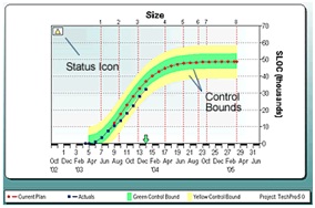
Regardless of whether you use QSM default control limits or create your own control bound rules, SLIM-Control’s status icons help you instantly assess the status of various project metrics and take corrective action:

• When your actual data fall an average of one control bound from the plan, a green status icon lets you know the variation is within acceptable limits. When calculating the average distance from the plan, SLIM-Control® considers all data points but gives more weight to the later data points.
• When actual data average 1-2 control bounds from the plan, a yellow (warning) status icon is shown. The yellow icon alerts the user that the displayed metric needs to be monitored closely.
• When the data points average more than 2 control bounds from the plan, a red status icon will be displayed to indicate that re-planning may be needed. The user can generate a new forecast to completion to learn the impact of current deviations upon the delivery date.

The Scoreboard Summary Report can even create an audit trail for key project metrics over time:

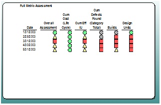
Need more information before making a decision? SLIM-Control’s Snapshot Manager records the status (green, yellow, or red) of various metrics as the project unfolds. This time series view adds context to your analysis: if a “red” metric has consistently lagged behind the plan, it’s probably time to take corrective action. If the same metric has stayed in the green region for the entire project, a red status icon could alert you to a possible data entry error.

SLIM-Control’s customizable control bounds, status icons, and snapshot manager make tracking and monitoring projects a snap!

The first step is recognizing duplicate projects.  There are two ways this is done:

• If the project was created in SLIM-WebServices, it contains a unique identifyer.  Two projects with the same unique identifyer are tagged as duplicates.
•  If the project originated with SLIM-Suite, if the internal ID and the Project Name match it is considered a duplicate.

Prior to reading the import file, you are presented with a screen to select one of three options for handling duplicate projects:

• Import Duplicates - import all projects from the source database.
• Skip Duplicates - import only non-duplicate projects from the source database.
• Update Duplicates - replace existing projects with matching projects from the source database.

Is there a limit on the number of projects that can be loaded into SLIM-MasterPlan?

There is no limit to the number of projects you can load into MasterPlan other than what is allowed by the graphics and memory capabilities of your PC. But if your MasterPlan workbook includes an unusually large number of projects it may be difficult to see all the projects clearly on graphs.

Here are some suggestions for MasterPlan files with a large number of projects:

• Place a single graph on each view to allow more room for MasterPlan to display the projects onscreen.
• Use the Level of Detail tab in Gantt Chart Properties to adjust the number of levels shown
• Group your projects by category, perhaps by division, year, budget, or program to make your MasterPlan estimates more meaningful
• Consider moving projects which are more similar to iterations to SLIM-Estimate as a Work Breakdown Structure (WBS)

No.  The Utilities are available on the Support | Downloads page.  Contact QSM Support to obtain the username and password.

You may have up to 20 custom menu items.

It is a single-level menu only.  You cannot create submenues.

View the Reports and Graphs Export Table to see the best way to get SLIM-Suite reports and graphs into other applications.

There's a good fit between my total defect data and the plan but in the defects by category charts, the defect actuals for each category aren't tracking the plan very well. How can I fix this?

Chances are your defect category percentages need to be adjusted. To tune these percentages using your actual data, create a Multi-Metric Time Series Chart and insert a QSM Tracked Defects Category Total (Actual) metric for each defect category you're tracking:

Next, right click on your chart to access the chart property tabs. On the Data tab, select "Percent of first metric's data points" and click OK to exit the dialog.

Next, toggle your Multi-Metric chart into report form:

If the weekly or monthly values seem fairly consistent, you can simply use the latest % of total for each category. If you see a lot of variation, you may want to average the values - don't be afraid to experiment until you get the best visual fit! Enter the % for each category on the Reliability tab of the Project Environment dialog:

Once you return to the defects by category views, you should see a better fit between the plan and actuals.

My actual defect data points don't show up on the defect remaining and defect remaining/sloc reports and graphs.   Why not?

Before we can calculate and display the number of errors remaining, we must know the forecasted number of errors in the system.  Planned defects remaining is the difference between planned total defects and planned defects found at various points in time. Actual defects remaining are calculated by subtracting actual defects found from the forecasted total defects.

Therefore, the actual number of defects remaining will be shown only when a forecast exists.

The Solution Panel says my peak staff value is 10.3, but the Average Staffing Rate charts and reports show a peak staff of 10.1. What is causing this inconsistency?

The theoretical Rayleigh curve used to derive the values on the Solution Panel is a smooth curve resulting in different staffing numbers at each point along the x-axis. In drawing the Average Staffing chart, this smooth theoretical curve is approximated by a series of discrete staffing rates (with one bar, or average staffing rate value, per month).

The graph and solution panel values won't always match exactly because the graphical peak staff is always taken mid-month for any internal month while the solution panel always shows the highest peak staff point on the staffing curve (regardless of when it occurs). Usually the theoretical curve does not peak exactly at mid-month, so the true peak shown on the solution panel will not match the one on the average staffing charts unless the theoretical peak happens to fall at mid-month.

On large projects where a longer schedule allows a natural smoothing of the staffing curve, the theoretical peak staff will usually be close to the average staff rate value. On shorter projects, you can expect to see larger discrepancies.

When I change the Person Hours per Person Month field in Accounting Options, there is no change to the total schedule and effort for the project.  How can I adjust the estimate to reflect overtime?

The person hours/person month field was never intended to be used for performing time/effort tradeoffs.  For estimating purposes, SLIM-Estimate assumes that a FTE person is a FTE person, regardless of the number of hours in an effort month.  To account for overtime or unusual staffing situations, you should adjust the FTE (full-time equivalent) peak staffing level.  

For example, to reflect 10% overtime, you need a peak staff that is 1.1 times the current peak.  You can do this using the Control Panel peak staffing dial or by extending or shortening the Phase 3 schedule.

NOTE: if you are using a PI from your completed projects, you should only make this type of adjustment if your history does not include overtime.  It is usually better to be conservative in making adjustments as overtime hours are often less productive.  If the completed projects you used to derive a PI had a similar amount of overtime, it is already reflected in the PI and no adjustment is needed.  

Sometimes the effort data points on my Life Cycle Sensitivity to PI graph have values that do not always increase (or decrease); e.g., there are small dips in the data.

Remember that the time and effort shown on these graphs are life cycle values. The most likely cause of slight variations in the expected behavior of the data is caused by variation in the effort for phase 4. Staffing projections for phase 4 are dependent on the staffing rate at the end of phase 3. Therefore, differences in the final phase 3 staffing rate can result in variations in the total effort for phase 4. You can check to see if this is the case by making the solutions in question the current solution, then comparing the phase 4 effort in the solution panel of the staffing view.

What is the impact of selecting various phase staffing shapes? When should I deviate from the default Rayleigh pattern, and how is my estimate affected?

We have found that the default Rayleigh pattern is the staffing pattern that best matches the application of effort to the work to be performed but due to staffing constraints or different software management styles, you may decide that another staffing pattern fits your organization or project better.

In general, the various staffing shapes can be described as follows: 

• Front Load Rayleigh peaks at approximately 40% the phase 
• Medium Front Load Rayleigh peaks midway through the phase 
• Medium Rear Load Rayleigh peaks at approximately 75% of the phase 
• Rear Load Rayleigh (Phase 3 only) peaks at the end of the phase 
• Level Load maintains a constant staffing level over the entire phase
• Exponential (Phase 4 only) gives the most rapid drop off of staffing from the end of Phase 3.
• Stair Step (Phase 4 only) begins at about half of the staffing level from the end of Phase 3 and stair steps down.
• Straight Line: (Phase 4 only) represents a straight-line decrease in staffing from the end of Phase 3.
• Rayleigh (Phase 4 only) is a natural tailing off/continuation of any Phase 3 Rayleigh curve. Not valid if the selected Phase 3 staffing shape is Level Load. 

Level loading is generally seen in the development of very small systems. In larger systems, early application of people often represents wasted effort. The Default Rayleigh shape determines the staffing shape based on the size of the application. QSM has found that small projects (less than 18,000 lines of code) tend to have a Front Load Rayleigh profile while larger systems (greater than 100,000 lines of code) typically reach peak staffing towards the end of phase 3. For very small systems (3 to 6 months in duration with a peak staff of 1-3 persons), a level load profile is more appropriate.

The estimated total effort for each of the staffing patterns for the first three phases will remain constant regardless of the pattern selected. Phase 4 effort will vary, depending on the shape of phase 3. This is because in phase 4, manpower tails off from the final Phase 3 staffing level and is therefore a function of the number of people on board at the end of phase 3 and the length of phase 4. Projects that peak at the end of Phase 3 will have higher phase 4 effort. Projects that peak earlier will have lower phase 4 effort.

If you are using default QSM overlaps for the phases, you can expect to see some differences in the phase overlap when you change the staffing pattern. This occurs because SLIM attempts to produce the smoothest aggregate staffing pattern when moving from one phase to the next.

For example, the overlap percentage between Phases 2 and 3 will be 0% if Phase 3 is Level Loaded. Otherwise the overlap ratio will range from  33% to 40% as the phase 2 staffing shape changes from Front Load Rayleigh to Medium Front Load Rayleigh.

Is there a limit on the number of projects that can be loaded into SLIM-MasterPlan?

There is no limit to the number of projects you can load into MasterPlan other than what is allowed by the graphics and memory capabilities of your PC. But if your MasterPlan workbook includes an unusually large number of projects it may be difficult to see all the projects clearly on graphs.

Here are some suggestions for MasterPlan files with a large number of projects:

• Place a single graph on each view to allow more room for MasterPlan to display the projects onscreen.
• Use the Level of Detail tab in Gantt Chart Properties to adjust the number of levels shown
• Group your projects by category, perhaps by division, year, budget, or program to make your MasterPlan estimates more meaningful
• Consider moving projects which are more similar to iterations to SLIM-Estimate as a Work Breakdown Structure (WBS)

My current plan is extremely inconsistent with my actual data. For instance, the project started a year late and has already slipped by almost 15 months.  Using my original plan, the actual defect data yields a defect tuning factor of 2000% when I run the Defect Tuning Calculator function. 

Is the plan being factored into the defect tuning calculations? If so, can significant variation between the plan and the actuals result in an incorrect tuning factor?

When looking for the best tuning factor, SLIM-Control must make some assumptions in order to generate a set of theoretical defect curves and find the one that best fits your actual data. If these assumptions are incorrect (for example, if either the expected phase 3 duration or expected effort are wrong) then any calculations based on these assumptions will be affected. 

Before running the Defect Tuning Calculator, it’s a good idea to review the current plan to ensure reasonable consistency with your actual data. If your actuals have diverged significantly from the current plan, it should be updated before defect tuning is performed. To update the current plan, run a forecast, make the forecast the current plan, then re-run the Defect Tuning Calculator. 

The planned MTTD value shown on my graph for the final month of phase 3 is not the same as the value reported in the Project Profile report and the consistency report for my Phase 3 MTTD. It appears to be slightly higher in the reports.  Why?

The value displayed on graphs is the average MTTD rate for the final month of phase 3, but the MTTD value reported in the reports represents the planned MTTD at the end of phase 3. You should expect this value to be somewhat higher than the average value for the entire month, because the theoretical MTTD is always improving (getting larger) as time progresses.

My actual defect data points don't show up on the defect remaining and defect remaining/sloc reports and graphs.   Why not?

Before we can calculate and display the number of errors remaining, we must know the forecasted number of errors in the system.  Planned defects remaining is the difference between planned total defects and planned defects found at various points in time. Actual defects remaining are calculated by subtracting actual defects found from the forecasted total defects.

Therefore, the actual number of defects remaining will be shown only when a forecast exists.

I changed my runtime environment from 5 days to 7 days. I would have expected my MTTD value to get smaller because I am running the system longer. Why did my MTTD value get larger?

The MTTD value is simply the reciprocal of the monthly defect rate. Suppose the expected defect rate is 100 defects found during the last month of phase 3. This is a theoretical monthly rate number based on an average runtime environment. The MTTD for this month is therefore 1 month/100 errors or .01 months between defects. 

Because it is difficult to think in terms of .01 months, you can specify a more intuitive MTTD time unit.  If you select days, then .01 months is the same as .01 * 30 (roughly) or .3 days between defects (assuming you are running 7 days a week). However, if you are running only 5 days a week, then .01 months converts to (.01 * 20) or .2 days.

I sometimes get poor defect curve fits when running a forecast.  What can I do to improve this?

Getting a good curve fit is important - the poorer the fit, the less confidence you will have in the projected new time for that set of data. The goodness of fit is particularly important during the latter stages of Phase 3 because defect data is weighted more heavily at that time. There are two things you can do to improve your defect curve fits:

1.  Assess the reliability of early data points carefully. If you have little confidence in the earliest defect data, you should throw it out. Our theoretical defect data curve algorithm assumes defects are being captured from the start of Phase 3 in a consistent and systematic manner. In practice, however, systematic logging of defects is often not performed until around Systems Integration Test (71% of phase 3 duration). If your early defect data is very erratic, chances are those data points are unreliable. If you know (or suspect) this to be the case, exclude the unreliable data points from curve fitting and forecasting. Unreliable data introduces random noise into SLIM-Control's calculations and creates unreliable forecasts.

2.  Try to determine the best tuning factor for your defect data. This is fairly easy to do once any early noisy data points have been discarded. There are two ways to get a handle on the defect tuning factor.  You can use either one, or combine the two methods:

• The first method uses past projects to generate a historic defect tuning factor. You can use any similar projects captured in SLIM-DataManager. Individual defect tuning factors for each project can be displayed on DataManager’s Project List View by selecting Tools | Customize View Layout from the menu. To get the average Defect Tuning Factor for one or more completed projects, import them into SLIM-Control using the History | Load Projects menu item and then run the Defect Tuning Calculator.  If you plan on using an average DTF from your history, you may wish to inspect the data and eliminate outliers to prevent distortion of the average.
• Once you have entered at least three actual total defect data points into SLIM-Control the Defect Tuning Calculator can also calculate a defect tuning factor from your actual defect data.

Once the expected defect total has been tuned to your history or actual data, you should see an improvement in your defect curve fits. If you’re tracking Defects Found by Category, here's one final step that will help ensure optimal curve fits:

• Tune the % of total defects for each category using your actual data. For more information on how to do this, see the FAQ entitled, "How Do I Tune My Defect Category Percentages?".

If you are still getting poor data fits after performing the steps outlined above, either try to determine the reasons or simply exclude defect data from the forecast curve fit.

My actual MTTD data points start at different times depending on whether there is a forecast being displayed. Why?

MTTD is not truly relevant until the entire system is integrated and functioning as a complete entity.  For this reason, MTTD values are not shown until Systems Integration Test (which occurs at about 71% of phase 3).   

Because we do not know the actual phase 3 time until the system is completed, we show actual MTTD data points starting at the same time as the plan unless there is a forecast present. Planned MTTD data points will always begin at about 71% of the planned phase 3 time. 

Once a forecast is present, the actual/forecast MTTD data points will be shown starting at 71% of the forecasted phase 3 time.

I’d like my MTTD forecasts to reflect the number of test hours for each reporting period. How do I do this in SLIM-Control?

The Weighted MTTD option allows you to account for the actual hours spent testing each reporting period. Often the number of test hours fluctuates from month to month, causing large swings or "find and fix cycles" as test effort is directed to finding defects one period, then drops off as effort goes into fixing newly discovered defects during the next period. Using the Weighted MTTD option will smooth out these "find and fix" cycles, giving you a smoother defect curve.  Be sure to click the box at the top of the Metric Definitions dialog box in order to display both active and inactive metrics.

To use the Weighted MTTD metric, you must activate it by choosing Tools | Customize Metric Definitions from the menu. Locate the active defect metrics folder (Hint: the folder title will be bolded). If you don't see the metric, make sure you are displaying all active and inactive metrics. Scroll down and select the Weighted MTTD metric, then click the Edit Metric button:

Activate the metric by checking the “Active” checkbox and click OK to exit.

Next, activate the QSM Test folder. Note the lack of bold type – this category is inactive by default. Select the folder title and activate the category using the Edit Category button:

Click OK to save your changes and exit the Metrics Definitions dialogs.

The number of testing hours per reporting period should now appear on the Metrics tab of the Actual Data screen (select Control | Actual Data from the menu). As with all custom metrics, the testing hours field is appended to the list of standard metrics so you will need to scroll down to the bottom of the metric list to see the Test Hours field. This is where you will enter the actual hours spent testing for each reporting period.

This error is a message generated by the DAO Engine. It occurs when input exceeds the maximum size for the database field we’re trying to write to.  Please contact QSM Support if you see this error message.

How do I set Phase Start dates?

Phase start dates, duration, and effort settings are used to configure the lifecycle model to your development methods and practices.  Select Estimate | Solution Assumptions from the main menu, then select the Phase Tuning tab.  The start date for the first phase included in the project is the project start date specified on the Solution Assumptions Basic Info tab or via Solution Wizards.

Subsequent phases can be set to begin at:

• Ratio - a specific percentage of the prior phase’s duration (most common)
• Fixed Overlap - a specified number of months into the prior phase
• Specific Date - a specific date.

Select Tuning Factor History... to use phase tuning data from select completed projects loaded in your SLIM-Estimate workbook.

How can I change the unit for Total system size in the Balanced Risk and other solution wizards? Currently it is set to IU, but we use Function Points.

Solution wizards that require a size estimate assumption use the Sizing By History technique to obtain an initial "ballpark" estimate based on the statistical size ranges, or t-shirt sizes, in your project's associated trend group(s).  This technique uses the Function Unit and Gearing Factor in the Project Environment settings.  Most of the templates installed with SLIM-Suite have the Function Unit set to the Base Size Unit, either IU or SLOC.  

To change the Function Unit to Stories, Features, Function Points, or other size unit, select Tools | Customize Project Environment from the menu. On the Project Description Tab, there is a Function Unit list box.  Select Function Points or other unit, then enter an appropriate Gearing Factor to represent the average number of Base Size Units (elementary programming steps) contained in your selected  Function Unit (ex.: a gearing factor of 50 represents 50 Base Size Units per Function Point).  

If you need help determining an appropriate gearing factor, visit the Function Point Gearing Factors page on the QSM web site, download our Gearing Factors whitepaper, or contact QSM for assistance.

View the Reports and Graphs Export Table to see the best way to get SLIM-Suite reports and graphs into other applications.

There's a good fit between my total defect data and the plan but in the defects by category charts, the defect actuals for each category aren't tracking the plan very well. How can I fix this?

Chances are your defect category percentages need to be adjusted. To tune these percentages using your actual data, create a Multi-Metric Time Series Chart and insert a QSM Tracked Defects Category Total (Actual) metric for each defect category you're tracking:

Next, right click on your chart to access the chart property tabs. On the Data tab, select "Percent of first metric's data points" and click OK to exit the dialog.

Next, toggle your Multi-Metric chart into report form:

If the weekly or monthly values seem fairly consistent, you can simply use the latest % of total for each category. If you see a lot of variation, you may want to average the values - don't be afraid to experiment until you get the best visual fit! Enter the % for each category on the Reliability tab of the Project Environment dialog:

Once you return to the defects by category views, you should see a better fit between the plan and actuals.

My current plan is extremely inconsistent with my actual data. For instance, the project started a year late and has already slipped by almost 15 months.  Using my original plan, the actual defect data yields a defect tuning factor of 2000% when I run the Defect Tuning Calculator function. 

Is the plan being factored into the defect tuning calculations? If so, can significant variation between the plan and the actuals result in an incorrect tuning factor?

When looking for the best tuning factor, SLIM-Control must make some assumptions in order to generate a set of theoretical defect curves and find the one that best fits your actual data. If these assumptions are incorrect (for example, if either the expected phase 3 duration or expected effort are wrong) then any calculations based on these assumptions will be affected. 

Before running the Defect Tuning Calculator, it’s a good idea to review the current plan to ensure reasonable consistency with your actual data. If your actuals have diverged significantly from the current plan, it should be updated before defect tuning is performed. To update the current plan, run a forecast, make the forecast the current plan, then re-run the Defect Tuning Calculator. 

I sometimes get poor defect curve fits when running a forecast.  What can I do to improve this?

Getting a good curve fit is important - the poorer the fit, the less confidence you will have in the projected new time for that set of data. The goodness of fit is particularly important during the latter stages of Phase 3 because defect data is weighted more heavily at that time. There are two things you can do to improve your defect curve fits:

1.  Assess the reliability of early data points carefully. If you have little confidence in the earliest defect data, you should throw it out. Our theoretical defect data curve algorithm assumes defects are being captured from the start of Phase 3 in a consistent and systematic manner. In practice, however, systematic logging of defects is often not performed until around Systems Integration Test (71% of phase 3 duration). If your early defect data is very erratic, chances are those data points are unreliable. If you know (or suspect) this to be the case, exclude the unreliable data points from curve fitting and forecasting. Unreliable data introduces random noise into SLIM-Control's calculations and creates unreliable forecasts.

2.  Try to determine the best tuning factor for your defect data. This is fairly easy to do once any early noisy data points have been discarded. There are two ways to get a handle on the defect tuning factor.  You can use either one, or combine the two methods:

• The first method uses past projects to generate a historic defect tuning factor. You can use any similar projects captured in SLIM-DataManager. Individual defect tuning factors for each project can be displayed on DataManager’s Project List View by selecting Tools | Customize View Layout from the menu. To get the average Defect Tuning Factor for one or more completed projects, import them into SLIM-Control using the History | Load Projects menu item and then run the Defect Tuning Calculator.  If you plan on using an average DTF from your history, you may wish to inspect the data and eliminate outliers to prevent distortion of the average.
• Once you have entered at least three actual total defect data points into SLIM-Control the Defect Tuning Calculator can also calculate a defect tuning factor from your actual defect data.

Once the expected defect total has been tuned to your history or actual data, you should see an improvement in your defect curve fits. If you’re tracking Defects Found by Category, here's one final step that will help ensure optimal curve fits:

• Tune the % of total defects for each category using your actual data. For more information on how to do this, see the FAQ entitled, "How Do I Tune My Defect Category Percentages?".

If you are still getting poor data fits after performing the steps outlined above, either try to determine the reasons or simply exclude defect data from the forecast curve fit.

I’d like my MTTD forecasts to reflect the number of test hours for each reporting period. How do I do this in SLIM-Control?

The Weighted MTTD option allows you to account for the actual hours spent testing each reporting period. Often the number of test hours fluctuates from month to month, causing large swings or "find and fix cycles" as test effort is directed to finding defects one period, then drops off as effort goes into fixing newly discovered defects during the next period. Using the Weighted MTTD option will smooth out these "find and fix" cycles, giving you a smoother defect curve.  Be sure to click the box at the top of the Metric Definitions dialog box in order to display both active and inactive metrics.

To use the Weighted MTTD metric, you must activate it by choosing Tools | Customize Metric Definitions from the menu. Locate the active defect metrics folder (Hint: the folder title will be bolded). If you don't see the metric, make sure you are displaying all active and inactive metrics. Scroll down and select the Weighted MTTD metric, then click the Edit Metric button:

Activate the metric by checking the “Active” checkbox and click OK to exit.

Next, activate the QSM Test folder. Note the lack of bold type – this category is inactive by default. Select the folder title and activate the category using the Edit Category button:

Click OK to save your changes and exit the Metrics Definitions dialogs.

The number of testing hours per reporting period should now appear on the Metrics tab of the Actual Data screen (select Control | Actual Data from the menu). As with all custom metrics, the testing hours field is appended to the list of standard metrics so you will need to scroll down to the bottom of the metric list to see the Test Hours field. This is where you will enter the actual hours spent testing for each reporting period.

The Installation and Deployment section of the QSM Resource Library web page provides System Requirements, step by step installation instructions, and other useful information about SLIM-Suite.

Information on the latest version of SLIM-Suite (along with download links, release notes, and installation instructions) can be found on the Installation and Upgrades page of the QSM website.  To see whether you're running the latest version, select Help | Check for updates from the menu of any SLIM-Suite application.

Often SLIM-Suite license renewals do not correspond with new product releases.  To update the license information for your current SLIM-Suite installation, use Windows Control Panel | Programs and Features application utililty.  Select the appropriate QsmTools installation (e.g. QsmTools 10.3) and right-click and choose Change.  Select Modify on the Install Shield screen and follow the prompts to enter your new Registration Code and Activation Code(s).  Review the list of products to be installed to ensure they match your license agreement.

No.  When the server copy of SLIM-Suite is updated, all users are automatically upgraded to the same version of SLIM-Suite.  No further action is needed on your part.

You can find the username and password in the following places:

1. Your license or upgrade email you received at the beginning of your license period.

• If you are upgrading from a prior version of SLIM Suite 8.1, there should be a readme.txt file in your Tools81 directory. The default path for this directory is c:/Program Files (x86)/QSM/Tools81, but you can also find it by right clicking any SLIM-Suite application shortcut and looking at the shortcut properties.

Note that versions 8.0 and 8.1 have their own, version specific license codes - to install version 8.1, you will need a set of 8.1 license codes. If you cannot locate any of these documents or have questions, please contact your software administrator or email QSM support.

There are two possibilities here:

• Your license codes have expired. Check the expiration date on your license email to make sure the license codes you’re using are still valid.
• You’re using license codes from a prior or different version of SLIM-Suite. License codes are version specific, so make sure the version number in your license email matches the version you’re installing. If you need help, contact your Account Manager or email QSM support.

To open the workbook, first make sure you are running the latest version of SLIM-Suite.

• If you have not yet installed the latest release, visit the upgrades page and download the latest version. You'll need license registration and activation codes for the latest release (see your license email). Not sure if you have the latest release? You can check for updates right from the Help menu in any SLIM-Suite application.
• If you have already installed the latest version, check to make sure you don't have multiple versions of the applications on your machine (ex: version 8.0 and version 8.1). If you are running multiple versions of SLIM-Suite, opening workbooks from the File menu (File | Open…) will help to avoid confusion between the different versions.

Yes. Because SLIM-Suite 8.1 and 8.2 each have their own license codes, install to separate application folders, and maintain their own registry entries and support files, they can be installed and run on the same machine.

No. Because SLIM-Suite workbooks are database files, workbooks created in newer versions often contain fileds and data that did not exist in earlier versions of the tools. For this reason, SLIM-Suite workbooks cannot "revert back" to older file formats.

Yes. SLIM-Suite workbook files are forward, but not backward, compatible. This means that earlier version workbooks can be opened and upgraded using the latest version of SLIM-Suite. Once a workbook has been upgraded, it can no longer be used with earlier versions of SLIM-Suite.

List of features and fixes for version 8.1b7.
List of features and fixes for version 8.1a.
List of features and fixes for version 8.0g2.
List of features and fixes 8.0a-g.

 A checksum error occurs when the values you entered for company name and location don't match the values expected by the setup program. For example, if your license email shows the Company name as "Dan's Software Emporium" and you type in "Dans Software Emporium", setup will detect the missing apostrophe in "Dans" and return a checksum error. If you pasted license information from your license email into the Setup dialogs, check to make sure you didn't inadvertently capture/paste any leading or trailing spaces. If you require assistance, please email us.

This deployment whitepaper answers common questions asked by SLIM-Suite users. If you have additional questions or would like to discuss your deployment options in greater detail, please contact QSM support.

Download the 8.1 installation manual.
Download the 8.2 installation manual.
Download the 9.0 installation manual.
Contact QSM support.

If you are upgrading from a prior version of SLIM Suite 8.1, there should be a readme.txt file in your Tools81 directory. The default path for this directory is c:/Program Files(x86)/QSM/Tools81, but you can also find it by right clicking any SLIM 81 application shortcut and looking at the shortcut properties.  In most instances, you will not need this information to upgrade to the latest release of version 8.1.

Your activation code, installation instructions, and license information can also be found in your version 8.1 QSM license or upgrade email.

If you need help locating these documents, please contact your software administrator or email QSM support.

User documentation in pdf and online help form are installed with the products. Online help is available via the Help menu in SLIM-Suite.

User Guides are installed (optionally) in pdf format. Version 8.1 user guides are installed to the Tools81 Documentation folder located under MyDocuments on your machine. Version 8.0 user guides are installed to your Tools80 application directory.  If you accepted the default installation location during setup, this will be C:\Program Files(x86)\QSM\Tools80\Doc.

Here's how to locate your SLIM license information:

• If the applications are already installed:
  • Simply launch any SLIM application and look at the right side of the splash screen, or
  • With the application open, select Help | About SLIM... from the menu to access the splash screen.

• If your license has expired or the application has not been installed yet, try the following:
  •  If the application is installed on your computer, simply browse to the directory where it is installed (Usually C:\Program Files\QSM\Toolsnn, where “nn” is the current version of SLIM-Suite). To determine the path to the application directory, right-click on the application shortcut and select the "properties" tab. Locate the readme.txt file located in your Toolsnn folder. Open this file in Notepad or any other text editor - it contains your license information.
  • If the applications have not yet been installed, contact the software administrator for your company and ask for a copy of your license email.
  • If you need help locating your software administrator or license email (or if you have questions) call QSM at 800 424-6755 for assistance.

What are the latest versions of the SLIM Tool Suite?

Information on the latest version of SLIM-Suite (along with download links, release notes, and installation FAQs) can be found on the Downloads page of the QSM website. To see whether you're running the latest version, select Help | Check for updates from the menu of any SLIM-Suite application.

The Installation and Deployment section of the QSM Resource Library web page provides System Requirements, step by step installation instructions, and other useful information about SLIM-Suite.

Information on the latest version of SLIM-Suite (along with download links, release notes, and installation instructions) can be found on the Installation and Upgrades page of the QSM website.  To see whether you're running the latest version, select Help | Check for updates from the menu of any SLIM-Suite application.

No.  When the server copy of SLIM-Suite is updated, all users are automatically upgraded to the same version of SLIM-Suite.  No further action is needed on your part.

What are the latest versions of the SLIM Tool Suite?

Information on the latest version of SLIM-Suite (along with download links, release notes, and installation FAQs) can be found on the Downloads page of the QSM website. To see whether you're running the latest version, select Help | Check for updates from the menu of any SLIM-Suite application.

When I change the Person Hours per Person Month field in Accounting Options, there is no change to the total schedule and effort for the project.  How can I adjust the estimate to reflect overtime?

The person hours/person month field was never intended to be used for performing time/effort tradeoffs.  For estimating purposes, SLIM-Estimate assumes that a FTE person is a FTE person, regardless of the number of hours in an effort month.  To account for overtime or unusual staffing situations, you should adjust the FTE (full-time equivalent) peak staffing level.  

For example, to reflect 10% overtime, you need a peak staff that is 1.1 times the current peak.  You can do this using the Control Panel peak staffing dial or by extending or shortening the Phase 3 schedule.

NOTE: if you are using a PI from your completed projects, you should only make this type of adjustment if your history does not include overtime.  It is usually better to be conservative in making adjustments as overtime hours are often less productive.  If the completed projects you used to derive a PI had a similar amount of overtime, it is already reflected in the PI and no adjustment is needed.  

Sometimes the effort data points on my Life Cycle Sensitivity to PI graph have values that do not always increase (or decrease); e.g., there are small dips in the data.

Remember that the time and effort shown on these graphs are life cycle values. The most likely cause of slight variations in the expected behavior of the data is caused by variation in the effort for phase 4. Staffing projections for phase 4 are dependent on the staffing rate at the end of phase 3. Therefore, differences in the final phase 3 staffing rate can result in variations in the total effort for phase 4. You can check to see if this is the case by making the solutions in question the current solution, then comparing the phase 4 effort in the solution panel of the staffing view.

When I change the Person Hours per Person Month field on the Accounting tab of the Solution Assumptions dialog, there is no change to the total schedule and effort for the project. Why is this?

Many SLIM-Estimate and SLIM-Control users have asked why their overall schedule does not change when they change the value of the "Person Hours per Person Month" field,  Solution Assumptions screen, Accounting Tab.

The number of Person Hours comprising a particular organization's Person Month is not used to calculate total effort.  If your chosen effort unit is Person Months, the hours per month setting is not used at all. If, on the other hand, your effort unit is weeks, days, or hours, your hours per month will be used to convert the estimated total effort (in Person Months) into your chosen effort unit.

At first, this may seem counter-intuitive. Shouldn't an increase or decrease in the number of Person Hours in a Person Month be reflected in the final estimate?

The number of staff hours in an organization's staffing month is more relevant in the accounting world than it is in software estimation. It attempts to account for items such as vacations, meetings, and administrative activities but in most cases, it is merely an estimate or average.  It may tell how many hours will be charged to a particular project, but has nothing to say about how much is actually accomplished during those hours (or even how many actual hours were worked). The productivity index, or PI, is where actual work produced is measured.

The Productivity Index, or PI, reflects a number of environmental factors such as:

If you are using a PI calculated from your past projects, your user-specified PI already reflects the conditions in your working environment. Holding other factors constant, organizations which have high "administrative overhead" will tend to have a lower calculated productivity index than organizations which maximize time spent working on the most productive project tasks.

SLIM-Estimate® is a macro model based on the software equation described in Measures for Excellence. The SLIM software equation is designed to estimate consistently across a broad spectrum of working environments and accounting standards. For this reason, the effort parameter was originally calculated in Person Years, which are converted to Person Months in SLIM-Estimate. Once the total effort in PM has been determined, it can be converted into your chosen effort unit for display on charts and reports.  But what if you have no historical data and are using the PI suggested by the QSM database? SLIM estimating and project control tools will still give you a good first estimate that you can continue to refine as more project data becomes available. As projects are completed, SLIM tools will calculate the project PI's from your historical data. These PI's can be used to calibrate new estimates to the unique conditions in your development environment.

As you begin to compare and analyze PI's from completed projects, you can spot and eliminate bottlenecks as well as identify successful strategies that you can repeat to improve productivity. Storing project metrics in a useful and accessible form and analyzing them to identify trends is the key to process and productivity improvement. Consistent use of SLIM tools results in increasingly accurate estimates and will help you build a repository of historical data for future analysis and benchmarking.

I need a gearing factor for a language not listed on the Function Point Languages Table.  Is this information available from QSM?  What are my options if QSM does not have this information?

Although the Function Point Languages Table is fairly extensive, we do not always have enough information to provide gearing factors for every language. Before we can use a completed project in our Gearing Factors table, certain conditions must be satisified:

1.  The project must be sized in function points.  Although thousands of projects in our database are sized in function points, we are starting with a subset of a subset of the database.
2. The project must be recent.  Because coding techniques and languages change over time, we would not want to include projects that were 20 years old.
3. The project must be developed in a single language or the requested language must comprise at least 80 to 90% of the project.  These days, however, it’s not uncommon for projects to be developed with a mix of technologies and languages. A project that contains only 20% Oracle  should not be used to determine an Oracle gearing factor.
4. There should be a decent sample size.  A large sample size gives more reliable and realistic gearing factor information than a very small sample size.

Given these constraints, if you do not see a language listed in the Function Point Languages Table,  consider using the higher level language as a starting point and adjust your risk.  For example, if you were searching for an APEX (Oracle) gearing factor but did not see that language listed in the table, you can start with the gearing factor for Oracle (or another similar language) and adjust the uncertainty on size to build an appropriate amount of risk buffer into your estimate.

If you would like to know if QSM has any information about a specific language’s gearing factor, please e-mail QSM support.

What is the purpose of the gearing factor?

Gearing factors are used to convert projects with many different sizing units (objects, modules, or use cases for example) back to a common sizing unit: the Basic Work Unit. The Basic Work Unit represents the smallest sizing unit that is common to all projects.

This conversion is important for two reasons. First, it allows us to apply the same family of PIs (or Productivity Indices) to all projects. Second, it allows you to compare your project, whether it is sized in tables, screens, or any other sizing unit, to QSM’s industry – or your own custom - trend lines, which can be sized in a variety of size units.

In our research, we have found a strong correlation between system size and important metrics like PI, schedule, effort, and defects. For more information on gearing factors, download our free whitepaper.

Can I use the forecast function to explore various staffing options?

When you run a forecast, SLIM-Control bases the future staffing profile on the peak staff and staffing shape defined in the current plan.

While Phase 3 is ongoing, run a tradeoff forecast to see the impact of increasing or decreasing staff and apply any resulting schedule tradeoff to your existing forecast.  To run a tradeoff forecast, select Control | Tradeoff Forecast… from the menu.

Once Phase 3 has completed, use the maintenance forecast to evaluate staff tradeoffs.  The maintenance forecast can only be performed during Phase 4.  To run a maintenance forecast, select Control | Run Forecast… from the menu.

Why don't my staffing rate numbers add up to the same total shown on cumulative effort charts and reports?

First, it is important to understand the difference between the average staffing rate and cumulative effort charts and reports.

Average Staffing Rate charts and reports display the number of FTE staff used by the project during any given month, regardless of how much of the month is covered by that phase. When a phase starts or ends mid-month, the staffing rate for that month is not affected.  

Cumulative Effort charts and reports display the total effort for each month.   So here, when a phase starts or ends mid-month, the total effort reflects those partial months.

To see this more clearly, let's look at an example.  If there 10 people work during December (and the phase begins on December 31st), then the Staffing Rate chart and report will show 10 people for December; but the Cumulative Effort for that month would only be .33 mm (10 people x .033 months). This logic holds true for other rate values like defects and cost.

A second factor that may cause discrepancies between cumulative effort or cost and the sum of the monthly effort/cost rates is really a calculus issue.  Staffing numbers represent the average manpower rate for a given time period. These numbers are typically taken at mid-month. 

For graphing purposes, it is more practical to break up the smooth theoretical curve used to derive cumulative effort/cost into slices (like bars in a histogram) where the top of each bar corresponds to the average staffing rate for each month. Because each bar has a flat top, each month a small amount of error is introduced as there will always be a small area under the curve that is not covered by the bars.

As we add more and more months (bars) to the staffing chart, the bars become narrower and narrower and the amount of error decreases. If the intervals are small enough, the sum of the rates should be very close to the cumulative effort. However, when the intervals are large (for instance, monthly for a 3-month project), the approximation will not be as close. 

The Solution Panel says my peak staff value is 10.3, but the Average Staffing Rate charts and reports show a peak staff of 10.1. What is causing this inconsistency?

The theoretical Rayleigh curve used to derive the values on the Solution Panel is a smooth curve resulting in different staffing numbers at each point along the x-axis. In drawing the Average Staffing chart, this smooth theoretical curve is approximated by a series of discrete staffing rates (with one bar, or average staffing rate value, per month).

The graph and solution panel values won't always match exactly because the graphical peak staff is always taken mid-month for any internal month while the solution panel always shows the highest peak staff point on the staffing curve (regardless of when it occurs). Usually the theoretical curve does not peak exactly at mid-month, so the true peak shown on the solution panel will not match the one on the average staffing charts unless the theoretical peak happens to fall at mid-month.

On large projects where a longer schedule allows a natural smoothing of the staffing curve, the theoretical peak staff will usually be close to the average staff rate value. On shorter projects, you can expect to see larger discrepancies.

When I change the Person Hours per Person Month field in Accounting Options, there is no change to the total schedule and effort for the project.  How can I adjust the estimate to reflect overtime?

The person hours/person month field was never intended to be used for performing time/effort tradeoffs.  For estimating purposes, SLIM-Estimate assumes that a FTE person is a FTE person, regardless of the number of hours in an effort month.  To account for overtime or unusual staffing situations, you should adjust the FTE (full-time equivalent) peak staffing level.  

For example, to reflect 10% overtime, you need a peak staff that is 1.1 times the current peak.  You can do this using the Control Panel peak staffing dial or by extending or shortening the Phase 3 schedule.

NOTE: if you are using a PI from your completed projects, you should only make this type of adjustment if your history does not include overtime.  It is usually better to be conservative in making adjustments as overtime hours are often less productive.  If the completed projects you used to derive a PI had a similar amount of overtime, it is already reflected in the PI and no adjustment is needed.  

What is the impact of selecting various phase staffing shapes? When should I deviate from the default Rayleigh pattern, and how is my estimate affected?

We have found that the default Rayleigh pattern is the staffing pattern that best matches the application of effort to the work to be performed but due to staffing constraints or different software management styles, you may decide that another staffing pattern fits your organization or project better.

In general, the various staffing shapes can be described as follows: 

• Front Load Rayleigh peaks at approximately 40% the phase 
• Medium Front Load Rayleigh peaks midway through the phase 
• Medium Rear Load Rayleigh peaks at approximately 75% of the phase 
• Rear Load Rayleigh (Phase 3 only) peaks at the end of the phase 
• Level Load maintains a constant staffing level over the entire phase
• Exponential (Phase 4 only) gives the most rapid drop off of staffing from the end of Phase 3.
• Stair Step (Phase 4 only) begins at about half of the staffing level from the end of Phase 3 and stair steps down.
• Straight Line: (Phase 4 only) represents a straight-line decrease in staffing from the end of Phase 3.
• Rayleigh (Phase 4 only) is a natural tailing off/continuation of any Phase 3 Rayleigh curve. Not valid if the selected Phase 3 staffing shape is Level Load. 

Level loading is generally seen in the development of very small systems. In larger systems, early application of people often represents wasted effort. The Default Rayleigh shape determines the staffing shape based on the size of the application. QSM has found that small projects (less than 18,000 lines of code) tend to have a Front Load Rayleigh profile while larger systems (greater than 100,000 lines of code) typically reach peak staffing towards the end of phase 3. For very small systems (3 to 6 months in duration with a peak staff of 1-3 persons), a level load profile is more appropriate.

The estimated total effort for each of the staffing patterns for the first three phases will remain constant regardless of the pattern selected. Phase 4 effort will vary, depending on the shape of phase 3. This is because in phase 4, manpower tails off from the final Phase 3 staffing level and is therefore a function of the number of people on board at the end of phase 3 and the length of phase 4. Projects that peak at the end of Phase 3 will have higher phase 4 effort. Projects that peak earlier will have lower phase 4 effort.

If you are using default QSM overlaps for the phases, you can expect to see some differences in the phase overlap when you change the staffing pattern. This occurs because SLIM attempts to produce the smoothest aggregate staffing pattern when moving from one phase to the next.

For example, the overlap percentage between Phases 2 and 3 will be 0% if Phase 3 is Level Loaded. Otherwise the overlap ratio will range from  33% to 40% as the phase 2 staffing shape changes from Front Load Rayleigh to Medium Front Load Rayleigh.

View the Reports and Graphs Export Table to see the best way to get SLIM-Suite reports and graphs into other applications.

There's a good fit between my total defect data and the plan but in the defects by category charts, the defect actuals for each category aren't tracking the plan very well. How can I fix this?

Chances are your defect category percentages need to be adjusted. To tune these percentages using your actual data, create a Multi-Metric Time Series Chart and insert a QSM Tracked Defects Category Total (Actual) metric for each defect category you're tracking:

Next, right click on your chart to access the chart property tabs. On the Data tab, select "Percent of first metric's data points" and click OK to exit the dialog.

Next, toggle your Multi-Metric chart into report form:

If the weekly or monthly values seem fairly consistent, you can simply use the latest % of total for each category. If you see a lot of variation, you may want to average the values - don't be afraid to experiment until you get the best visual fit! Enter the % for each category on the Reliability tab of the Project Environment dialog:

Once you return to the defects by category views, you should see a better fit between the plan and actuals.

The planned MTTD value shown on my graph for the final month of phase 3 is not the same as the value reported in the Project Profile report and the consistency report for my Phase 3 MTTD. It appears to be slightly higher in the reports.  Why?

The value displayed on graphs is the average MTTD rate for the final month of phase 3, but the MTTD value reported in the reports represents the planned MTTD at the end of phase 3. You should expect this value to be somewhat higher than the average value for the entire month, because the theoretical MTTD is always improving (getting larger) as time progresses.

Sometimes, one or more of the menu items in SLIM-Control are grayed out and I'm not sure why.

Grayed out menu options generally denote features that will not become available until some condition has been satisfied. Here are some of the most common reasons a menu option may be unavailable:

1.     You're trying to edit a QSM Default custom metric or control bound. Since QSM default custom metrics and control bound definitions cannot be edited, the options for these metrics are grayed out. You can, however,  copy a QSM default metric or control bound definition and edit the copy.

2.     You're trying to enter actual data for a metric that has not started yet or is complete. Before you can enter actual data for a metric, you must first enter an actual start date for that metric. Likewise, once you've entered an actual end date for a metric, you will no longer be able to enter actual data for that metric. 

3.     You're trying to set a start or end date for a metric that is tied to a phase:  Start and end date fields for planned staffing/effort are disabled because staffing and effort data is always tied to a specific phase. For example, phase 2 effort begins on the first day of phase 2 and ends on the last day of phase 2. Start/end dates for each phase are defined on the Phases tab of the Plan property sheet (Control | Plan Data). 

Start dates for Defect metrics are customizable, but defect end dates are disabled because they coincide with the end of the life cycle.

4.     You're trying to enter a start or end date for an inactive phase. On the Plan | Phases tab, planned start or end dates can only be entered for active phases. To view/edit the active phases for the project, select Tools | Customize Project Environment and select the Phases tab.

When I change the Person Hours per Person Month field in Accounting Options, there is no change to the total schedule and effort for the project.  How can I adjust the estimate to reflect overtime?

The person hours/person month field was never intended to be used for performing time/effort tradeoffs.  For estimating purposes, SLIM-Estimate assumes that a FTE person is a FTE person, regardless of the number of hours in an effort month.  To account for overtime or unusual staffing situations, you should adjust the FTE (full-time equivalent) peak staffing level.  

For example, to reflect 10% overtime, you need a peak staff that is 1.1 times the current peak.  You can do this using the Control Panel peak staffing dial or by extending or shortening the Phase 3 schedule.

NOTE: if you are using a PI from your completed projects, you should only make this type of adjustment if your history does not include overtime.  It is usually better to be conservative in making adjustments as overtime hours are often less productive.  If the completed projects you used to derive a PI had a similar amount of overtime, it is already reflected in the PI and no adjustment is needed.  

Sometimes the effort data points on my Life Cycle Sensitivity to PI graph have values that do not always increase (or decrease); e.g., there are small dips in the data.

Remember that the time and effort shown on these graphs are life cycle values. The most likely cause of slight variations in the expected behavior of the data is caused by variation in the effort for phase 4. Staffing projections for phase 4 are dependent on the staffing rate at the end of phase 3. Therefore, differences in the final phase 3 staffing rate can result in variations in the total effort for phase 4. You can check to see if this is the case by making the solutions in question the current solution, then comparing the phase 4 effort in the solution panel of the staffing view.

What is the impact of selecting various phase staffing shapes? When should I deviate from the default Rayleigh pattern, and how is my estimate affected?

We have found that the default Rayleigh pattern is the staffing pattern that best matches the application of effort to the work to be performed but due to staffing constraints or different software management styles, you may decide that another staffing pattern fits your organization or project better.

In general, the various staffing shapes can be described as follows: 

• Front Load Rayleigh peaks at approximately 40% the phase 
• Medium Front Load Rayleigh peaks midway through the phase 
• Medium Rear Load Rayleigh peaks at approximately 75% of the phase 
• Rear Load Rayleigh (Phase 3 only) peaks at the end of the phase 
• Level Load maintains a constant staffing level over the entire phase
• Exponential (Phase 4 only) gives the most rapid drop off of staffing from the end of Phase 3.
• Stair Step (Phase 4 only) begins at about half of the staffing level from the end of Phase 3 and stair steps down.
• Straight Line: (Phase 4 only) represents a straight-line decrease in staffing from the end of Phase 3.
• Rayleigh (Phase 4 only) is a natural tailing off/continuation of any Phase 3 Rayleigh curve. Not valid if the selected Phase 3 staffing shape is Level Load. 

Level loading is generally seen in the development of very small systems. In larger systems, early application of people often represents wasted effort. The Default Rayleigh shape determines the staffing shape based on the size of the application. QSM has found that small projects (less than 18,000 lines of code) tend to have a Front Load Rayleigh profile while larger systems (greater than 100,000 lines of code) typically reach peak staffing towards the end of phase 3. For very small systems (3 to 6 months in duration with a peak staff of 1-3 persons), a level load profile is more appropriate.

The estimated total effort for each of the staffing patterns for the first three phases will remain constant regardless of the pattern selected. Phase 4 effort will vary, depending on the shape of phase 3. This is because in phase 4, manpower tails off from the final Phase 3 staffing level and is therefore a function of the number of people on board at the end of phase 3 and the length of phase 4. Projects that peak at the end of Phase 3 will have higher phase 4 effort. Projects that peak earlier will have lower phase 4 effort.

If you are using default QSM overlaps for the phases, you can expect to see some differences in the phase overlap when you change the staffing pattern. This occurs because SLIM attempts to produce the smoothest aggregate staffing pattern when moving from one phase to the next.

For example, the overlap percentage between Phases 2 and 3 will be 0% if Phase 3 is Level Loaded. Otherwise the overlap ratio will range from  33% to 40% as the phase 2 staffing shape changes from Front Load Rayleigh to Medium Front Load Rayleigh.

Is there a limit on the number of projects that can be loaded into SLIM-MasterPlan?

There is no limit to the number of projects you can load into MasterPlan other than what is allowed by the graphics and memory capabilities of your PC. But if your MasterPlan workbook includes an unusually large number of projects it may be difficult to see all the projects clearly on graphs.

Here are some suggestions for MasterPlan files with a large number of projects:

• Place a single graph on each view to allow more room for MasterPlan to display the projects onscreen.
• Use the Level of Detail tab in Gantt Chart Properties to adjust the number of levels shown
• Group your projects by category, perhaps by division, year, budget, or program to make your MasterPlan estimates more meaningful
• Consider moving projects which are more similar to iterations to SLIM-Estimate as a Work Breakdown Structure (WBS)

In SLIM-Suite, some dialog boxes are too large for my screen.  What is the recommended screen resolution?

If you are running at a low screen resolution, certain dialog boxes may not fit within the screen display. 

The recommended screen resolution is 1024 x 768 with 256 colors and 96 dpi (default small fonts). For optimal graphics display when running SLIM tools, the screen resolution should be set to at least 800 by 600 for small fonts (or at a higher resolution if you are using large fonts). 

My graph titles are being truncated in SLIM-Suite. Is there a way to fix this so that I can keep my chart title?

If a chart title or chart axis label is too long to fit in the allotted space, SLIM-Suite applications will truncate the text instead of wrapping to the next line. This happens on all QSM charts. There are a few options in this case:

• Reduce the font size.
• Shorten the title by cutting out words or using abbreviations.
• Maximize the display window.
• If the appearance is acceptable on printouts, leave the title as is.

To reduce the font size, select Tools | Customize Display | Screen/Printer Fonts, Colors, & Symbols.  On the Element side of the dialog box, select the desired chart title or label and click the Select Font… button to reduce the font size.