No software system of any realistic size is ever completely debugged—that is, error free

Edward Yourdon and Larry L. Constantine, 1975 1

The issue of software reliability was alive and well 20 years ago—and before that if memory serves.  Of course, the problem is still with us.  That makes it familiar and a fit subject for FMM-R.

Last year Yourdon wrote: “Defects are not the only measure of quality, of course; but they are the most visible indicator of quality throughout a project.” 2

Note his use of the word “throughout.” He did not say “at the end of the project” or “during integration test.”   Searching for defects throughout the entire development period is actually a familiar idea, too.  Michael Fagan codified the practice of early inspection in the 1970s. 3 Unfortunately, it is still not common practice.  It ought to be, agree all who have examined the data. To join this so far regrettably exclusive circle, you might start with Tom Gilb and Dorothy Graham’s thorough treatment. 4

Statistical control of defects

Statistical control of any attribute rests upon four footings. First, you have to have a metric. Well, we have that: number of defects, or more specifically, defects per month. You might have some technical problems defining just what a defect is, how many degrees of severity you want to use, what kind of paperwork (or, in deference to the computer, non-paperwork) you are going to record these defects on, and so on. These issues are solvable in principle, as many organizations have long since demonstrated.

Second, you need a means of projecting how frequently this attribute is going to turn up. It is that projection that you are, third, going to control against. By control, we simply mean comparing the actual number of defects you find each month against the projected number. If actuals are within a reasonable tolerance of projected values, you are on target. If actuals are outside the tolerance limits, fourth, do something!

Projecting defect rate

Getting that second foundation point, projecting the defect rate, has been something of a problem in software circles. It has not been for want of trying.

“Since the early 1970’s, several models have been proposed for estimating software reliability and some related parameters, such as mean time to failure (MTTF), residual error content, and other measures of confidence in the software,” reported C. V. Ramamoorthy and Farokh B. Bastani in a long survey paper in 1982. 5

 They unearthed 114 references!  Again, the idea of a reliability model has been around for a long time. It is familiar.

At about the same time, an industrial researcher, Marty Trachtenberg at RCA,

Moorestown, NJ, was searching for what he called “a practical reliability model.” 6 “Ensuring software reliability is currently the most critical unsolved problem in software engineering,” he said in the opening sentence of his article. Searching the literature, he found over 25 models.

“We were disappointed to find that the use of any of these models requires data known only after coding or testing begins,” he lamented, “when it is often too late to influence the software-engineering process in a cost-effective manner.”

In 1982, unfortunately for Trachtenberg, there was little data showing the rate of occurrence of defects over the entire life of software projects. After a search he found only 10 error histories. The individual histories were noisy.  There was little to suggest that some “invisible hand,” as Trachtenberg rather engagingly thought of a model, was shaping defect-rate behavior.

Fortunately, Trachtenberg was aware of a data manipulation process called “compositing.” It merged normalized data from all 10 histories into one histogram. It is a way of bringing out the pattern in noisy data.  Geophysical prospectors use compositing to bring out the detail in underground oil deposits.

“We found the suggestion of a Rayleigh curve,” Trachtenberg modestly reported. Then he found that Peter V. Norden had noted a Rayleigh curve in manpower employed on R & D projects, as we noted last month. And that we, ourselves, had confirmed the presence of the Rayleigh curve in software projects a few years earlier.

The Rayleigh defect-rate curve

Trachtenberg’s “suggestion” that there was a pattern in defect data and that it was Rayleigh-like in nature made sense to us. The staff rate followed a Rayleigh curve over the life of the project. The rate of committing errors was, we thought, very likely proportional to the rate of expending person hours, that is, people make “x” errors per hour of work. When they hurry, they probably make “x + y” errors per hour.  When the system is large and complex, they probably make still more errors per hour.  But when they work in a more productive, better organized operation, they may very well make fewer errors per hour.

All these factors—size, effort, development time, and process productivity—were already present in our software equation. It was only necessary for us to acquire some defect-rate data, and match it to these other four factors.  Then we could work out a defect-rate equation and curve.

Alas, we ran into the same problem that Trachtenberg had: there was at that time little defect-rate data spread over the entire course of development, from design to delivery and after.  However, there was lots of defect-rate data for the period of testing, shown in Figure 1.

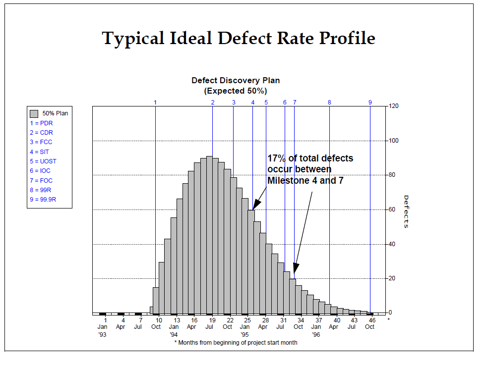
Hence, when we have a number for the defects detected during test, represented by the 17-percent area under the test portion of the curve, we can divide this number by 0.17 to get the expected total number of errors committed.  By the time the system gets to test, most of the errors have been corrected by inspections and unit test. Once we had the total number of errors (the area under the curve), we developed the defect-rate equation presented in Table 1.

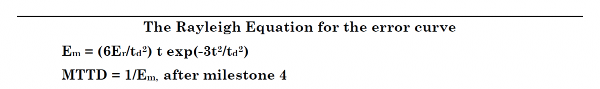
• E_r = Total number of errors expected over the life of the project
• E_m = Errors per month t = instantaneous elapsed time throughout the life cycle
• t_d = elapsed time at milestone 7, the 95% reliability level
• This time corresponds to the development time MTTD = Mean Time to Defect

[As a “get started” approximation for E_r, take the total number of of defects counted from the start of Systems Integration Test (MS4) to delivery (MS 7) and divide by 0.17. Systems used should be of similar size and the same application type as the system being estimated.]

In the last 10 years, of course, software organizations have recorded much more error data over the entire project period, enabling us to make the equation parameters more precise.  Even so, we have found that organizations differ perceptibly from the standard pattern.  To make their projections more accurate, they may fine tune them on the basis of defect data from their own past projects.

The main point of all this is: defects do follow a Rayleigh pattern, the same as effort, cost, and code constructed. This curve can be projected before the main build begins; it can be fine tuned.  It is the key ingredient for the statistical control of software reliability. All for now.

• 1. Edward Yourdon and Larry L. Constantine, Structured Design: Fundamentals of a Discipline of Computer Program and Systems Design, Prentice-Hall, Englewood Cliffs, NJ 1979. 473 pp.
• 2. Edward Yourdon, “Software Metrics,” Application Development Strategies (newsletter), Nov. 1994, 16 pp.
• 3. Michael E. Fagan, “Design and Code Inspections to Reduce Errors in Program Development,” IBM Systems Journal, 15 (3) 1976, pp. 182-211.
• 4. Tom Gilb and Dorothy Graham, Software Inspection, Addison-Wesley, Reading, MA.  1993, 471 pp.
• 5. C. V. Ramamoorthy and Farokh B. Bastani, “Software Reliability—Status and Perspectives,” IEEE Transactions on Software Engineering, Vol.  SE-8, No. 4 (July) 1982, pp. 354-371.
• 6. M. Trachtenberg, “Discovering how to ensure software reliability,” RCA Engineer, Jan.- Feb. 1982, pp. 53-57